Preconditioners — The Finite Element Method

The convergence rate of the conjugate gradient method is determined by the condition number of the matrix $A$ . The larger it is, the slower the method converges — many iterations are required to reach acceptable accuracy. The preconditioner $P$ is meant to improve this number by replacing the original system with an equivalent one with the matrix $P^{-1} \cdot A$ , whose eigenvalues should cluster in a narrow neighbourhood of one.

In practice there is no need to build $P^{-1} \cdot A$ explicitly: at every iteration it suffices to be able to solve the auxiliary problem

\displaystyle P \cdot z_k

\displaystyle = r_k,

(3.11)

using $z_k$ instead of the original residual $r_k$ — see formulas (3.7)–(3.8). Let us consider three variants.

1. No preconditioning ( $P$ $= I$ ). In this case $z_k$ $= r_k$ , and the method coincides with the classical conjugate gradient method. This variant is useful for debugging, but for ill-conditioned systems it converges slowly.

2. Jacobi preconditioner. As $P$ we take the diagonal part of the matrix $A$

\displaystyle P

\displaystyle = \operatorname{diag}(A)

\displaystyle = \operatorname{diag}(a_{11}, a_{22}, \ldots, a_{nn}).

(3.12)

Its application reduces to element-wise division

\displaystyle z_{k,\,i}

\displaystyle = \frac{r_{k,\,i}}{a_{ii}}.

(3.13)

This preconditioner is practically free in memory and time, but it takes into account only the diagonal, ignoring the couplings between the variables.

3. Incomplete Cholesky factorization (IC). For a symmetric positive definite matrix an approximate factorization is built

\displaystyle A

\displaystyle \approx L \cdot L^T,

(3.14)

where $L$ is a lower triangular matrix. Unlike the full Cholesky factorization, the fill-in elements in the positions of the original zeros are discarded — the nonzero structure of $L$ coincides with the structure of the lower triangle of $A$ . Once $L$ is built, applying the preconditioner consists of two triangular substitutions

\displaystyle L \cdot y

\displaystyle = r_k,

(3.15)

\displaystyle L^T \cdot z_k

\displaystyle = y.

(3.16)

Three variants of the preconditioner for the conjugate gradient method — **Fig. 3.3.** Preconditioners: identity ( $P$ $= I$ ), Jacobi ( $P$ $= \operatorname{diag}(A)$ ) and incomplete Cholesky ( $A$ $\approx L \cdot L^T$ ).

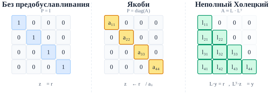
In FEM problems the incomplete Cholesky factorization usually gives the best trade-off: it is more expensive than the diagonal preconditioner (building $L$ and two triangular sweeps per iteration), but it noticeably reduces the number of iterations. For nonsymmetric or indefinite systems, which fall outside standard heat conduction problems, one should turn to the GMRES or BiCGSTAB methods with appropriate preconditioners.

This concludes the solution of sparse systems — next, let us talk about partitioning the geometry into simplices.