Simplices — The Finite Element Method

Before describing the solution, the domain on which it is sought must be partitioned into the simplest non-intersecting elements — simplices. The ways of building such partitions are discussed in detail in the chapter “Partitioning the geometry into simplices”, so here we only briefly recall the result we will rely on.

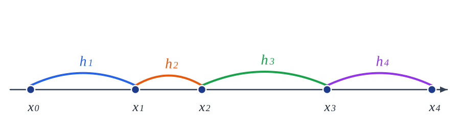
In the one-dimensional case the simplex is a segment. The interval $l$ on which the solution is sought is split into $n$ simplex segments $s_i, \; i$ $\in (1..n)$ ; unlike the finite difference method, their lengths may differ. The construction of these segments is described in the section “Segmentation”. An example is shown in figure Segment simplices: the length of simplex $s_2$ equals $x_2$ $- x_1$ .

Non-uniform one-dimensional segment simplices s₁…sₙ — **Fig. 5.1.** One-dimensional segment simplices $s_1, \ldots, s_n$ ; their lengths may differ.

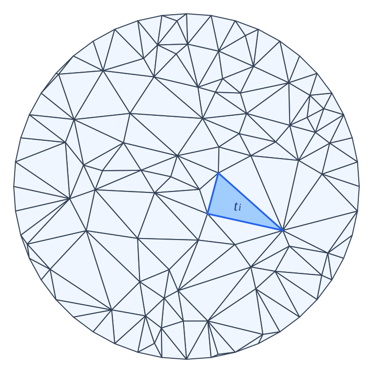
In the two-dimensional case the simplex is a triangle. The domain $S$ is partitioned into $n$ non-intersecting triangles $t_i, \; i$ $\in (1..n)$ by the constrained Delaunay triangulation — see the section “Triangulation”. An example is shown in figure Triangle simplices.

Triangulation of a convex circular domain — **Fig. 5.2.** A convex domain covered by non-intersecting triangle simplices (a real triangulation); one simplex is highlighted.

In the three-dimensional case the simplex is a tetrahedron. The domain $V$ is partitioned into $n$ non-intersecting tetrahedra $t_i, \; i$ $\in (1..n)$ ; the corresponding procedure is discussed in the section “Tetrahedralization”. The minimal simplex and its face-sharing neighbour are shown in figure Tetrahedron simplices.

Fig. 5.3. A tetrahedral simplex on vertices

p_1, \ldots, p_4

and its neighbour across the shared face (grey).

Once the domain is partitioned into simplices, the solution $\upsilon_h$ must be described on each of them.