M. Triangulation by divide and conquer

This appendix describes a triangulation algorithm following the divide-and-conquer scheme, with merging of sub-triangulations along common tangents. Historically it was the first one implemented in the project; the main text describes the currently used approach built on the CGAL library. The material below is kept as supplementary: it helps to understand the classical scheme and the difficulties with degenerate configurations that eventually led to the change of approach.

The basis is the divide-and-conquer algorithm from A. V. Skvortsov's monograph “Delaunay Triangulation and Its Applications”, with immediate Delaunay restructuring right after each new triangle is built. The algorithm has $O(N \log N)$ average- and worst-case complexity in the number of input points.

General scheme

The idea follows the classical divide-and-conquer paradigm.

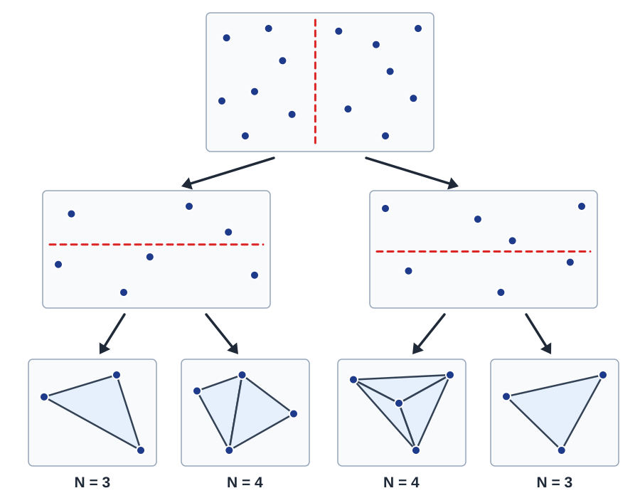
1. The point set is recursively split by a straight line into two roughly equal parts.
2. The recursion continues until each part contains three or four points — such configurations are triangulated explicitly.
3. The resulting sub-triangulations are pairwise stitched together along the common zone between their convex hulls.
4. During stitching, every new edge is checked against the Delaunay condition, and if necessary the pair of adjacent triangles is restructured by a diagonal swap.

Since any partial triangulation produced at intermediate recursion levels is a triangulation of the convex hull of the corresponding subset, the merge step always works with two convex regions. This greatly simplifies the search for tangents and the control of non-intersection.

Recursive point splitting

The split direction is chosen by the shape of the bounding rectangle: if it is wider than it is tall, the points are sorted and split by the horizontal coordinate, otherwise by the vertical one. This choice shortens the future seam between the sub-triangulations and therefore reduces the number of restructurings.

The sizes of the two parts are chosen so that all leaf subproblems have exactly three or four points. Large sets are split in half, while for a few small sizes a special “3 and $N$ $-3$” split is used, which guarantees that no leaf of the recursion ends up with one or two points. The correctness of this split for any $N$ $\geq 6$ follows from the fact that any $N$ is representable as $3k$, $3(k-1)$ $+4$ or $3(k-2)$ $+4 \cdot 2$.

In formalized form the recursive algorithm looks as follows.

1. If the number of points $N$ $= 3$, build a triangulation of a single triangle.
2. Otherwise, if $N$ $= 4$, build a triangulation of two or three triangles.
3. Otherwise, if $N$ $= 8$, split the set into two parts of four points each, apply the algorithm recursively and merge the results.
4. Otherwise, if $N$ $< 12$, split the set into parts of three and $N$ $-3$ points, apply the algorithm recursively and merge the results.
5. Otherwise ($N$ $\geq 12$) split the set in half, into parts of $\lfloor N/2 \rfloor$ and $\lceil N/2 \rceil$ points, apply the algorithm recursively and merge the results.

The recursion depth is $O(\log N)$, and the total work at each level is linear in the number of points, which gives the overall $O(N \log N)$ complexity in both the average and the worst case (figure Splitting).

Base configurations

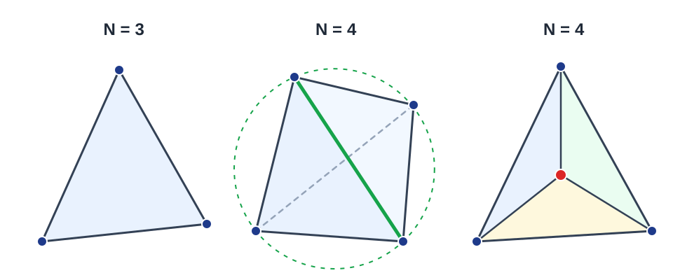
For three points there is a single admissible triangulation — one triangle built directly on those three vertices. For four points two cases are possible, depending on their relative position (figure Base cases).

1. All four points lie on the convex hull. The quadrilateral is split by one of its two diagonals. The choice is determined by the Delaunay condition: we check whether one of the vertices lies inside the circumscribed circle of the triangle built on the remaining three. The diagonal for which the condition holds is the one used in the base triangulation.
2. One point lies inside the triangle formed by the other three. The interior point is connected to each vertex of the outer triangle, splitting the region into three triangles.

Merging two sub-triangulations

Merging is the most substantial stage of the algorithm. Suppose we have left and right sub-triangulations, each a Delaunay triangulation of the convex hull of its points. The merge proceeds in three steps.

Finding common tangents. First, two common tangents — the lower and the upper — are found on the two convex hulls. An initial approximation is the edge connecting the rightmost point of the left hull with the leftmost point of the right hull; it is then iteratively advanced along the vertices of both hulls until it lies below (or above) all remaining points of the two sets. Between the two tangents remain two chains of boundary vertices — left and right — and the space between them is what has to be filled with triangles.

Filling the merge zone. The lower tangent is declared the current base edge. On both sides of it the nearest vertices of the two chains are taken, giving two candidates for the next triangle: one with the left vertex and one with the right. A candidate is admissible if it does not invert orientation (the interior angle at the base edge is less than straight) and does not cover already built parts of the mesh. If both candidates are admissible, the one with the larger minimal angle is chosen: such a triangle is “more equilateral” and less likely to be restructured later. The open side of the built triangle becomes the new base edge, and the step repeats until the base edge coincides with the upper tangent (figure Merge).

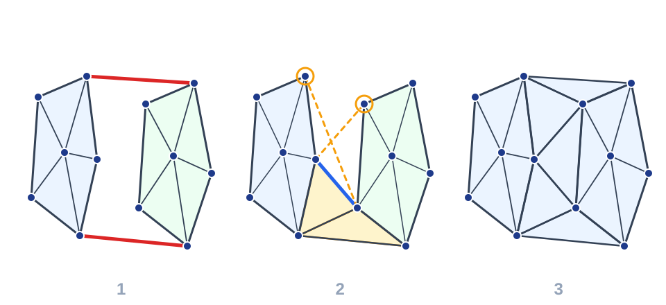
Immediate local restructuring. After a new triangle is added, its edges are checked against previously built neighbours: if the quadrilateral formed by the new triangle and its edge neighbour violates the Delaunay condition, a flip is performed. Immediate restructuring removes the need for a separate final pass over the mesh and usually reduces the total number of restructurings.

Inserting constraint edges

The algorithm above builds the Delaunay triangulation of the convex hull of the points but knows nothing about domain boundaries and hole contours. To guarantee that prescribed edges are present in the mesh, they are inserted into the finished triangulation by a separate edge-recovery operation.

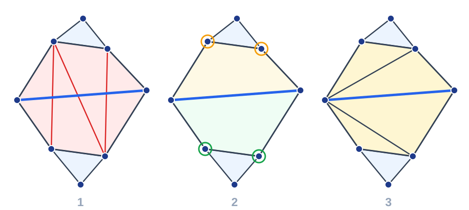
A single edge is inserted as follows: all triangles crossed by the segment are found and removed — this leaves a polygonal cavity in the mesh, which the inserted segment splits into two chains of vertices, an upper and a lower one; each chain is independently re-filled with triangles, and the edge ends up in the mesh (figure Edge insertion). After insertion the edge is marked as a constraint: flipping across it is forbidden, so no later restructuring can destroy it, while the Delaunay condition near it may legitimately be violated.

In the current version of the project this very operation is performed by CGAL (the insert_constraint method), but the logic inside is the same.

Why the scheme was abandoned

The divide-and-conquer scheme relies on building convex hulls, finding tangents and controlling orientation — all these operations reduce to sign predicates evaluated in floating-point arithmetic. On “good” inputs (in general position) this works, but on regular, axis-aligned data typical of a square computational domain, degenerate configurations arise: many points on one vertical or horizontal line (collinearity) and rectangular quadruples of points lying on one circle (cocircularity). In these cases the predicate value is an exact zero, while floating-point evaluation yields noise of arbitrary sign instead. The tangent search and the merge start to contradict themselves: flat (zero-area) “fan” triangles appear along the boundary and the Delaunay condition is violated. These are precisely the difficulties that led to the switch to the library-based approach with exact predicates described in the main text.