Boundary conditions

The equation alone is not enough: it only describes the relations between the particles of the object itself, but the object does not exist like a spherical horse in a vacuum, so the object under study must somehow be connected to the surrounding world. The boundary value conditions for our example are the combination of the boundary conditions and the initial condition $T_0(M)$. The initial condition is clear: it describes the temperature in the object $M$ at all interior points and on the boundary $S$. There may be a case where the boundary is not explicitly specified: for example, we compute the electromagnetic field above the ground; clearly the domain under consideration is the whole Universe, but we artificially bound it within some reasonable limits and adapt the size of the finite elements in proportion to the distance from the field source. This is an example of the advantage of FEM over FDM, where we would have to compute the field where it is of little interest to us. I will also note that we will not specify the thermal conductivity coefficients or the density function — all of this will be in the most general form that FEM can accept; the type of boundary condition, for example, directly affects the construction of the method and must not be overlooked.

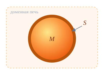
The initial condition is clear, so let us move on to the boundary conditions. Imagine that we heat a steel ball in a blast furnace at 1000 K; we can assume the ball is placed in an environment on which it has no influence, and the sphere bounding it will stay at 1000 K throughout the heating cycle. Such conditions are described by equation (1.13$\displaystyle T(M, t)$ $\displaystyle = \Phi(M, t), \quad M$ $\displaystyle \in S.$), which is called a boundary condition of the first kind, or a Dirichlet boundary condition:

That is, the temperature on the surface is prescribed by some function, which in general may depend on time; a particular case is a constant (in our example, 1000 K).

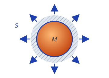
Now let us take the ball out of the furnace heated to 1000 K and wrap it in thermal insulation. The ball will cool at roughly one rate, that is, the cooling pace will be more or less constant. This is a boundary condition of the second kind (Neumann); it prescribes the normal heat flux through the surface (1.14$\displaystyle \lambda \cdot \frac{\partial T(M, t)}{\partial \vec{n}}$ $\displaystyle = \Phi(M, t), \quad M$ $\displaystyle \in S,$):

where $\vec{n}$ is the outward normal to the surface $S$ at the point $M$, $\lambda$ is the thermal conductivity. This condition applies when the surface is being heated or cooled: if $\Phi(M, t)$ $\equiv 0$, the surface is insulated; if $\Phi(M, t)$ $< 0$, cooling takes place; if $\Phi(M, t)$ $> 0$, heating.

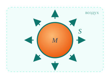
There is also a condition of the third kind (Robin). Let the same ball cool in the open air with no wind: heat is gradually removed from the surface into the environment, the more intensely the hotter the ball is relative to the air. Such heat exchange is described by equation (1.15$\displaystyle -\lambda \cdot \frac{\partial T(M, t)}{\partial \vec{n}}$ $\displaystyle = \alpha \left( T(M, t) - T_c \right), \quad M$ $\displaystyle \in S,$):

where $\alpha$ is the heat transfer coefficient, $T_c$ is the ambient temperature. The flux through the surface is proportional to the temperature difference — this is Newton's law of cooling.

In this guide we restrict ourselves to the first two kinds of boundary conditions.

The corresponding homogeneous boundary conditions have the form

The importance of homogeneous boundary conditions will become apparent later, when we obtain the general solution by the Fourier method of separation of variables.

Equation (1.8$\displaystyle \frac{\partial T(M, t)}{\partial t}$ $\displaystyle = a^2 \cdot \Delta T(M, t)$ $\displaystyle + f(M, t),$) with the initial condition $T_0(M)$ and the boundary condition (1.13$\displaystyle T(M, t)$ $\displaystyle = \Phi(M, t), \quad M$ $\displaystyle \in S.$) is called the Dirichlet boundary value problem, while the same equation with the same initial condition but with the boundary condition (1.14$\displaystyle \lambda \cdot \frac{\partial T(M, t)}{\partial \vec{n}}$ $\displaystyle = \Phi(M, t), \quad M$ $\displaystyle \in S,$) is called the Neumann boundary value problem. We will consider both problems in this guide.