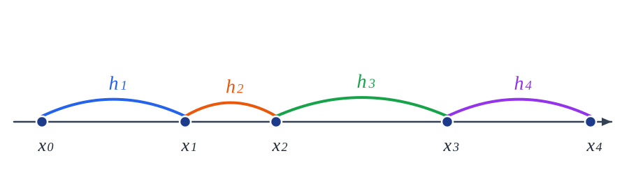
Let us see how the Bubnov–Galerkin functional from Appendix I works in practice: we go through a one-dimensional example from start to finish — from the test functions to the system of linear equations in matrix form.
We solve the heat equation L [ u ] L[u] = f {} = f L L = ∂ u ∂ t {} = \frac{\partial u}{\partial t} − a 2 Δ u {} - a^2 \Delta u [ x 0 , x 4 ] [x_0, x_4] 1.14 λ ⋅ ∂ T ( M , t ) ∂ n → \displaystyle \lambda \cdot \frac{\partial T(M, t)}{\partial \overrightarrow{n}} = Φ ( M , t ) , \displaystyle {} = \Phi(M, t), M \displaystyle M ∈ S , \displaystyle {} \in S, ∂ u ∂ n ∣ x = x 0 \frac{\partial u}{\partial n}\bigg|_{x=x_0} = g 0 {} = g_0 ∂ u ∂ n ∣ x = x 4 \frac{\partial u}{\partial n}\bigg|_{x=x_4} = g 4 {} = g_4
Fig. J.1. The example mesh: four simplex segments s 1 , … , s 4 s_1, \ldots, s_4 x 0 , … , x 4 x_0, \ldots, x_4 l ( i ) ( i + 1 ) l_{(i)(i+1)} Take four simplex segments s 1 , s 2 , s 3 , s 4 s_1, s_2, s_3, s_4 x 1 , x 2 , x 3 x_1, x_2, x_3 x 0 , x 4 x_0, x_4 Figure J.1 ). The test functions on the simplex segments take the form
υ ( 0 ) ( 1 ) ( x ) \displaystyle \upsilon_{(0)(1)}(x) = q 0 ⋅ ϕ 0 ( x ) \displaystyle {} = q_0 \cdot \phi_0(x) + q 1 ⋅ ϕ 1 ( x ) \displaystyle {} + q_1 \cdot \phi_1(x) υ ( 1 ) ( 2 ) ( x ) \displaystyle \upsilon_{(1)(2)}(x) = q 1 ⋅ ϕ 1 ( x ) \displaystyle {} = q_1 \cdot \phi_1(x) + q 2 ⋅ ϕ 2 ( x ) \displaystyle {} + q_2 \cdot \phi_2(x) υ ( 2 ) ( 3 ) ( x ) \displaystyle \upsilon_{(2)(3)}(x) = q 2 ⋅ ϕ 2 ( x ) \displaystyle {} = q_2 \cdot \phi_2(x) + q 3 ⋅ ϕ 3 ( x ) \displaystyle {} + q_3 \cdot \phi_3(x) υ ( 3 ) ( 4 ) ( x ) \displaystyle \upsilon_{(3)(4)}(x) = q 3 ⋅ ϕ 3 ( x ) \displaystyle {} = q_3 \cdot \phi_3(x) + q 4 ⋅ ϕ 4 ( x ) \displaystyle {} + q_4 \cdot \phi_4(x) The “hat” functions and their derivatives for the segment simplices are
ϕ 0 ( x ) \displaystyle \phi_0(x) = a 0 \displaystyle {} = a_0 + b 0 ⋅ x ϕ 0 ′ ( x ) \displaystyle {} + b_0 \cdot x \quad \phi_0'(x) = b 0 \displaystyle {} = b_0 ϕ 1 ( x ) \displaystyle \phi_1(x) = a 1 \displaystyle {} = a_1 + b 1 ⋅ x ϕ 1 ′ ( x ) \displaystyle {} + b_1 \cdot x \quad \phi_1'(x) = b 1 \displaystyle {} = b_1 ϕ 2 ( x ) \displaystyle \phi_2(x) = a 2 \displaystyle {} = a_2 + b 2 ⋅ x ϕ 2 ′ ( x ) \displaystyle {} + b_2 \cdot x \quad \phi_2'(x) = b 2 \displaystyle {} = b_2 ϕ 3 ( x ) \displaystyle \phi_3(x) = a 3 \displaystyle {} = a_3 + b 3 ⋅ x ϕ 3 ′ ( x ) \displaystyle {} + b_3 \cdot x \quad \phi_3'(x) = b 3 \displaystyle {} = b_3 ϕ 4 ( x ) \displaystyle \phi_4(x) = a 4 \displaystyle {} = a_4 + b 4 ⋅ x ϕ 4 ′ ( x ) \displaystyle {} + b_4 \cdot x \quad \phi_4'(x) = b 4 \displaystyle {} = b_4 The coefficients take the following values. Let us introduce the notation l ( i ) ( i + 1 ) l_{(i)(i+1)} = x i + 1 {} = x_{i+1} − x i {} - x_i x i x_i x i + 1 x_{i+1}
The hat-function coefficients for an arbitrary simplex between the points x i x_i x i + 1 x_{i+1}
a i \displaystyle a_i = x i + 1 l ( i ) ( i + 1 ) b i \displaystyle {} = \frac{\displaystyle x_{i+1}}{\displaystyle l_{(i)(i+1)}} \quad b_i = − 1 l ( i ) ( i + 1 ) \displaystyle {} = \frac{\displaystyle -1}{\displaystyle l_{(i)(i+1)}} a i + 1 \displaystyle a_{i+1} = − x i l ( i ) ( i + 1 ) b i + 1 \displaystyle {} = \frac{\displaystyle -x_i}{\displaystyle l_{(i)(i+1)}} \quad b_{i+1} = 1 l ( i ) ( i + 1 ) \displaystyle {} = \frac{\displaystyle 1}{\displaystyle l_{(i)(i+1)}} For the boundary hats ϕ 0 \phi_0 ϕ 4 \phi_4
Let us substitute the coefficients into the test functions and express them in terms of x x
For simplex s 1 s_1
υ ( 0 ) ( 1 ) ( x ) \displaystyle \upsilon_{(0)(1)}(x) = q 0 ⋅ ϕ 0 ( x ) \displaystyle {} = q_0 \cdot \phi_0(x) + q 1 ⋅ ϕ 1 ( x ) \displaystyle {} + q_1 \cdot \phi_1(x) = q 0 \displaystyle {} = q_0 ⋅ ( x 1 l ( 0 ) ( 1 ) − x l ( 0 ) ( 1 ) ) \displaystyle {} \cdot \left(\frac{\displaystyle x_1}{\displaystyle l_{(0)(1)}} - \frac{\displaystyle x}{\displaystyle l_{(0)(1)}}\right) + q 1 \displaystyle {} + q_1 ⋅ ( − x 0 l ( 0 ) ( 1 ) + x l ( 0 ) ( 1 ) ) \displaystyle {} \cdot \left(\frac{\displaystyle -x_0}{\displaystyle l_{(0)(1)}} + \frac{\displaystyle x}{\displaystyle l_{(0)(1)}}\right) = 1 l ( 0 ) ( 1 ) [ q 0 ⋅ ( x 1 − x ) + q 1 ⋅ ( x − x 0 ) ] \displaystyle {} = \frac{\displaystyle 1}{\displaystyle l_{(0)(1)}} \left[q_0 \cdot (x_1 - x) + q_1 \cdot (x - x_0)\right] For simplex s 2 s_2
υ ( 1 ) ( 2 ) ( x ) \displaystyle \upsilon_{(1)(2)}(x) = q 1 ⋅ ϕ 1 ( x ) \displaystyle {} = q_1 \cdot \phi_1(x) + q 2 ⋅ ϕ 2 ( x ) \displaystyle {} + q_2 \cdot \phi_2(x) = q 1 \displaystyle {} = q_1 ⋅ ( x 2 l ( 1 ) ( 2 ) − x l ( 1 ) ( 2 ) ) \displaystyle {} \cdot \left(\frac{\displaystyle x_2}{\displaystyle l_{(1)(2)}} - \frac{\displaystyle x}{\displaystyle l_{(1)(2)}}\right) + q 2 \displaystyle {} + q_2 ⋅ ( − x 1 l ( 1 ) ( 2 ) + x l ( 1 ) ( 2 ) ) \displaystyle {} \cdot \left(\frac{\displaystyle -x_1}{\displaystyle l_{(1)(2)}} + \frac{\displaystyle x}{\displaystyle l_{(1)(2)}}\right) = 1 l ( 1 ) ( 2 ) [ q 1 ⋅ ( x 2 − x ) + q 2 ⋅ ( x − x 1 ) ] \displaystyle {} = \frac{\displaystyle 1}{\displaystyle l_{(1)(2)}} \left[q_1 \cdot (x_2 - x) + q_2 \cdot (x - x_1)\right] For simplex s 3 s_3
υ ( 2 ) ( 3 ) ( x ) \displaystyle \upsilon_{(2)(3)}(x) = q 2 ⋅ ϕ 2 ( x ) \displaystyle {} = q_2 \cdot \phi_2(x) + q 3 ⋅ ϕ 3 ( x ) \displaystyle {} + q_3 \cdot \phi_3(x) = q 2 \displaystyle {} = q_2 ⋅ ( x 3 l ( 2 ) ( 3 ) − x l ( 2 ) ( 3 ) ) \displaystyle {} \cdot \left(\frac{\displaystyle x_3}{\displaystyle l_{(2)(3)}} - \frac{\displaystyle x}{\displaystyle l_{(2)(3)}}\right) + q 3 \displaystyle {} + q_3 ⋅ ( − x 2 l ( 2 ) ( 3 ) + x l ( 2 ) ( 3 ) ) \displaystyle {} \cdot \left(\frac{\displaystyle -x_2}{\displaystyle l_{(2)(3)}} + \frac{\displaystyle x}{\displaystyle l_{(2)(3)}}\right) = 1 l ( 2 ) ( 3 ) [ q 2 ⋅ ( x 3 − x ) + q 3 ⋅ ( x − x 2 ) ] \displaystyle {} = \frac{\displaystyle 1}{\displaystyle l_{(2)(3)}} \left[q_2 \cdot (x_3 - x) + q_3 \cdot (x - x_2)\right] For simplex s 4 s_4
υ ( 3 ) ( 4 ) ( x ) \displaystyle \upsilon_{(3)(4)}(x) = q 3 ⋅ ϕ 3 ( x ) \displaystyle {} = q_3 \cdot \phi_3(x) + q 4 ⋅ ϕ 4 ( x ) \displaystyle {} + q_4 \cdot \phi_4(x) = q 3 \displaystyle {} = q_3 ⋅ ( x 4 l ( 3 ) ( 4 ) − x l ( 3 ) ( 4 ) ) \displaystyle {} \cdot \left(\frac{\displaystyle x_4}{\displaystyle l_{(3)(4)}} - \frac{\displaystyle x}{\displaystyle l_{(3)(4)}}\right) + q 4 \displaystyle {} + q_4 ⋅ ( − x 3 l ( 3 ) ( 4 ) + x l ( 3 ) ( 4 ) ) \displaystyle {} \cdot \left(\frac{\displaystyle -x_3}{\displaystyle l_{(3)(4)}} + \frac{\displaystyle x}{\displaystyle l_{(3)(4)}}\right) = 1 l ( 3 ) ( 4 ) [ q 3 ⋅ ( x 4 − x ) + q 4 ⋅ ( x − x 3 ) ] \displaystyle {} = \frac{\displaystyle 1}{\displaystyle l_{(3)(4)}} \left[q_3 \cdot (x_4 - x) + q_4 \cdot (x - x_3)\right] Let us find the derivatives of the test functions with respect to x x
For simplex s 1 s_1
υ ( 0 ) ( 1 ) ′ ( x ) \displaystyle \upsilon'_{(0)(1)}(x) = 1 l ( 0 ) ( 1 ) ( q 1 − q 0 ) \displaystyle {} = \frac{\displaystyle 1}{\displaystyle l_{(0)(1)}} (q_1 - q_0) For simplex s 2 s_2
υ ( 1 ) ( 2 ) ′ ( x ) \displaystyle \upsilon'_{(1)(2)}(x) = 1 l ( 1 ) ( 2 ) ( q 2 − q 1 ) \displaystyle {} = \frac{\displaystyle 1}{\displaystyle l_{(1)(2)}} (q_2 - q_1) For simplex s 3 s_3
υ ( 2 ) ( 3 ) ′ ( x ) \displaystyle \upsilon'_{(2)(3)}(x) = 1 l ( 2 ) ( 3 ) ( q 3 − q 2 ) \displaystyle {} = \frac{\displaystyle 1}{\displaystyle l_{(2)(3)}} (q_3 - q_2) For simplex s 4 s_4
υ ( 3 ) ( 4 ) ′ ( x ) \displaystyle \upsilon'_{(3)(4)}(x) = 1 l ( 3 ) ( 4 ) ( q 4 − q 3 ) \displaystyle {} = \frac{\displaystyle 1}{\displaystyle l_{(3)(4)}} (q_4 - q_3) Let us compute the squares of the test functions:
For simplex s 1 s_1
υ ( 0 ) ( 1 ) 2 ( x ) \displaystyle \upsilon_{(0)(1)}^2(x) = 1 l ( 0 ) ( 1 ) 2 [ q 0 ⋅ ( x 1 − x ) + q 1 ⋅ ( x − x 0 ) ] 2 \displaystyle {} = \frac{\displaystyle 1}{\displaystyle l_{(0)(1)}^2} \left[q_0 \cdot (x_1 - x) + q_1 \cdot (x - x_0)\right]^2 = 1 l ( 0 ) ( 1 ) 2 [ q 0 2 ( x 1 − x ) 2 \displaystyle {} = \frac{\displaystyle 1}{\displaystyle l_{(0)(1)}^2} \bigl[ q_0^2(x_1 - x)^2 + 2 q 0 q 1 ( x 1 − x ) ( x − x 0 ) \displaystyle {} + 2q_0q_1(x_1 - x)(x - x_0) + q 1 2 ( x − x 0 ) 2 ] \displaystyle {} + q_1^2(x - x_0)^2 \bigr] For simplex s 2 s_2
υ ( 1 ) ( 2 ) 2 ( x ) \displaystyle \upsilon_{(1)(2)}^2(x) = 1 l ( 1 ) ( 2 ) 2 [ q 1 ⋅ ( x 2 − x ) + q 2 ⋅ ( x − x 1 ) ] 2 \displaystyle {} = \frac{\displaystyle 1}{\displaystyle l_{(1)(2)}^2} \left[q_1 \cdot (x_2 - x) + q_2 \cdot (x - x_1)\right]^2 = 1 l ( 1 ) ( 2 ) 2 [ q 1 2 ( x 2 − x ) 2 \displaystyle {} = \frac{\displaystyle 1}{\displaystyle l_{(1)(2)}^2} \bigl[ q_1^2(x_2 - x)^2 + 2 q 1 q 2 ( x 2 − x ) ( x − x 1 ) \displaystyle {} + 2q_1q_2(x_2 - x)(x - x_1) + q 2 2 ( x − x 1 ) 2 ] \displaystyle {} + q_2^2(x - x_1)^2 \bigr] For simplex s 3 s_3
υ ( 2 ) ( 3 ) 2 ( x ) \displaystyle \upsilon_{(2)(3)}^2(x) = 1 l ( 2 ) ( 3 ) 2 [ q 2 ⋅ ( x 3 − x ) + q 3 ⋅ ( x − x 2 ) ] 2 \displaystyle {} = \frac{\displaystyle 1}{\displaystyle l_{(2)(3)}^2} \left[q_2 \cdot (x_3 - x) + q_3 \cdot (x - x_2)\right]^2 = 1 l ( 2 ) ( 3 ) 2 [ q 2 2 ( x 3 − x ) 2 \displaystyle {} = \frac{\displaystyle 1}{\displaystyle l_{(2)(3)}^2} \bigl[ q_2^2(x_3 - x)^2 + 2 q 2 q 3 ( x 3 − x ) ( x − x 2 ) \displaystyle {} + 2q_2q_3(x_3 - x)(x - x_2) + q 3 2 ( x − x 2 ) 2 ] \displaystyle {} + q_3^2(x - x_2)^2 \bigr] For simplex s 4 s_4
υ ( 3 ) ( 4 ) 2 ( x ) \displaystyle \upsilon_{(3)(4)}^2(x) = 1 l ( 3 ) ( 4 ) 2 [ q 3 ⋅ ( x 4 − x ) + q 4 ⋅ ( x − x 3 ) ] 2 \displaystyle {} = \frac{\displaystyle 1}{\displaystyle l_{(3)(4)}^2} \left[q_3 \cdot (x_4 - x) + q_4 \cdot (x - x_3)\right]^2 = 1 l ( 3 ) ( 4 ) 2 [ q 3 2 ( x 4 − x ) 2 \displaystyle {} = \frac{\displaystyle 1}{\displaystyle l_{(3)(4)}^2} \bigl[ q_3^2(x_4 - x)^2 + 2 q 3 q 4 ( x 4 − x ) ( x − x 3 ) \displaystyle {} + 2q_3q_4(x_4 - x)(x - x_3) + q 4 2 ( x − x 3 ) 2 ] \displaystyle {} + q_4^2(x - x_3)^2 \bigr] Let us compute the squares of the derivatives of the test functions:
For simplex s 1 s_1
( υ ( 0 ) ( 1 ) ′ ( x ) ) 2 \displaystyle \left(\upsilon'_{(0)(1)}(x)\right)^2 = 1 l ( 0 ) ( 1 ) 2 ( q 1 − q 0 ) 2 \displaystyle {} = \frac{\displaystyle 1}{\displaystyle l_{(0)(1)}^2} (q_1 - q_0)^2 = 1 l ( 0 ) ( 1 ) 2 ( q 0 2 − 2 q 0 q 1 + q 1 2 ) \displaystyle {} = \frac{\displaystyle 1}{\displaystyle l_{(0)(1)}^2} \left(q_0^2 - 2q_0q_1 + q_1^2\right) For simplex s 2 s_2
( υ ( 1 ) ( 2 ) ′ ( x ) ) 2 \displaystyle \left(\upsilon'_{(1)(2)}(x)\right)^2 = 1 l ( 1 ) ( 2 ) 2 ( q 2 − q 1 ) 2 \displaystyle {} = \frac{\displaystyle 1}{\displaystyle l_{(1)(2)}^2} (q_2 - q_1)^2 = 1 l ( 1 ) ( 2 ) 2 ( q 1 2 − 2 q 1 q 2 + q 2 2 ) \displaystyle {} = \frac{\displaystyle 1}{\displaystyle l_{(1)(2)}^2} \left(q_1^2 - 2q_1q_2 + q_2^2\right) For simplex s 3 s_3
( υ ( 2 ) ( 3 ) ′ ( x ) ) 2 \displaystyle \left(\upsilon'_{(2)(3)}(x)\right)^2 = 1 l ( 2 ) ( 3 ) 2 ( q 3 − q 2 ) 2 \displaystyle {} = \frac{\displaystyle 1}{\displaystyle l_{(2)(3)}^2} (q_3 - q_2)^2 = 1 l ( 2 ) ( 3 ) 2 ( q 2 2 − 2 q 2 q 3 + q 3 2 ) \displaystyle {} = \frac{\displaystyle 1}{\displaystyle l_{(2)(3)}^2} \left(q_2^2 - 2q_2q_3 + q_3^2\right) For simplex s 4 s_4
( υ ( 3 ) ( 4 ) ′ ( x ) ) 2 \displaystyle \left(\upsilon'_{(3)(4)}(x)\right)^2 = 1 l ( 3 ) ( 4 ) 2 ( q 4 − q 3 ) 2 \displaystyle {} = \frac{\displaystyle 1}{\displaystyle l_{(3)(4)}^2} (q_4 - q_3)^2 = 1 l ( 3 ) ( 4 ) 2 ( q 3 2 − 2 q 3 q 4 + q 4 2 ) \displaystyle {} = \frac{\displaystyle 1}{\displaystyle l_{(3)(4)}^2} \left(q_3^2 - 2q_3q_4 + q_4^2\right) Let us write the linear approximation of the source function f ( x ) f(x) 6.36 e 1 \displaystyle e_1 = f i ⋅ x i + 1 − f i + 1 ⋅ x i x i + 1 − x i \displaystyle {} = \frac{\displaystyle f_i \cdot x_{i+1} - f_{i+1} \cdot x_i}{\displaystyle x_{i+1} - x_i} e 2 \displaystyle e_2 = f i + 1 − f i x i + 1 − x i \displaystyle {} = \frac{\displaystyle f_{i+1} - f_i}{\displaystyle x_{i+1} - x_i}
For simplex s 1 s_1 x 0 x_0 x 1 x_1
Since the heat source density function is identically zero on this interval:
f ~ ( 0 ) ( 1 ) ( x ) \displaystyle \widetilde{f}_{(0)(1)}(x) = 0. \displaystyle {} = 0. For simplex s 2 s_2 x 1 x_1 x 2 x_2
f ~ ( 1 ) ( 2 ) ( x ) \displaystyle \widetilde{f}_{(1)(2)}(x) = e 1 ( 1 ) ( 2 ) \displaystyle {} = e_1^{(1)(2)} + e 2 ( 1 ) ( 2 ) ⋅ x , \displaystyle {} + e_2^{(1)(2)} \cdot x, where:
e 1 ( 1 ) ( 2 ) \displaystyle e_1^{(1)(2)} = f 1 ⋅ x 2 − f 2 ⋅ x 1 x 2 − x 1 \displaystyle {} = \frac{\displaystyle f_1 \cdot x_2 - f_2 \cdot x_1}{\displaystyle x_2 - x_1} = f 1 ⋅ x 2 − f 2 ⋅ x 1 l ( 1 ) ( 2 ) \displaystyle {} = \frac{\displaystyle f_1 \cdot x_2 - f_2 \cdot x_1}{\displaystyle l_{(1)(2)}} e 2 ( 1 ) ( 2 ) \displaystyle e_2^{(1)(2)} = f 2 − f 1 x 2 − x 1 \displaystyle {} = \frac{\displaystyle f_2 - f_1}{\displaystyle x_2 - x_1} = f 2 − f 1 l ( 1 ) ( 2 ) \displaystyle {} = \frac{\displaystyle f_2 - f_1}{\displaystyle l_{(1)(2)}} For simplex s 3 s_3 x 2 x_2 x 3 x_3
f ~ ( 2 ) ( 3 ) ( x ) \displaystyle \widetilde{f}_{(2)(3)}(x) = e 1 ( 2 ) ( 3 ) \displaystyle {} = e_1^{(2)(3)} + e 2 ( 2 ) ( 3 ) ⋅ x , \displaystyle {} + e_2^{(2)(3)} \cdot x, where:
e 1 ( 2 ) ( 3 ) \displaystyle e_1^{(2)(3)} = f 2 ⋅ x 3 − f 3 ⋅ x 2 x 3 − x 2 \displaystyle {} = \frac{\displaystyle f_2 \cdot x_3 - f_3 \cdot x_2}{\displaystyle x_3 - x_2} = f 2 ⋅ x 3 − f 3 ⋅ x 2 l ( 2 ) ( 3 ) \displaystyle {} = \frac{\displaystyle f_2 \cdot x_3 - f_3 \cdot x_2}{\displaystyle l_{(2)(3)}} e 2 ( 2 ) ( 3 ) \displaystyle e_2^{(2)(3)} = f 3 − f 2 x 3 − x 2 \displaystyle {} = \frac{\displaystyle f_3 - f_2}{\displaystyle x_3 - x_2} = f 3 − f 2 l ( 2 ) ( 3 ) \displaystyle {} = \frac{\displaystyle f_3 - f_2}{\displaystyle l_{(2)(3)}} For simplex s 4 s_4 x 3 x_3 x 4 x_4
Since the heat source density function is identically zero on this interval:
f ~ ( 3 ) ( 4 ) ( x ) \displaystyle \widetilde{f}_{(3)(4)}(x) = 0. \displaystyle {} = 0. Now let us write the product of the source function and the corresponding test function for each simplex.
For simplex s 1 s_1
Since f ~ ( 0 ) ( 1 ) ( x ) \widetilde{f}_{(0)(1)}(x) = 0 {} = 0
f ~ ( 0 ) ( 1 ) ( x ) ⋅ υ ( 0 ) ( 1 ) ( x ) \displaystyle \widetilde{f}_{(0)(1)}(x) \cdot \upsilon_{(0)(1)}(x) = 0. \displaystyle {} = 0. For simplex s 2 s_2
f ~ ( 1 ) ( 2 ) ( x ) ⋅ υ ( 1 ) ( 2 ) ( x ) \displaystyle \widetilde{f}_{(1)(2)}(x) \cdot \upsilon_{(1)(2)}(x) = ( e 1 ( 1 ) ( 2 ) + e 2 ( 1 ) ( 2 ) ⋅ x ) \displaystyle {} = \left(e_1^{(1)(2)} + e_2^{(1)(2)} \cdot x\right) \quad ⋅ 1 l ( 1 ) ( 2 ) [ q 1 ⋅ ( x 2 − x ) + q 2 ⋅ ( x − x 1 ) ] . \displaystyle {} \cdot \frac{\displaystyle 1}{\displaystyle l_{(1)(2)}} \left[q_1 \cdot (x_2 - x) + q_2 \cdot (x - x_1)\right]. Substituting the values of e 1 ( 1 ) ( 2 ) e_1^{(1)(2)} e 2 ( 1 ) ( 2 ) e_2^{(1)(2)}
f ~ ( 1 ) ( 2 ) ( x ) ⋅ υ ( 1 ) ( 2 ) ( x ) \displaystyle \widetilde{f}_{(1)(2)}(x) \cdot \upsilon_{(1)(2)}(x) = 1 l ( 1 ) ( 2 ) 2 [ ( f 1 ⋅ x 2 − f 2 ⋅ x 1 ) + ( f 2 − f 1 ) ⋅ x ] \displaystyle {} = \frac{\displaystyle 1}{\displaystyle l_{(1)(2)}^2} \left[(f_1 \cdot x_2 - f_2 \cdot x_1) + (f_2 - f_1) \cdot x\right] \quad ⋅ [ q 1 ⋅ ( x 2 − x ) + q 2 ⋅ ( x − x 1 ) ] . \displaystyle {} \cdot \left[q_1 \cdot (x_2 - x) + q_2 \cdot (x - x_1)\right]. Let us transform the first factor:
( f 1 ⋅ x 2 − f 2 ⋅ x 1 ) \displaystyle (f_1 \cdot x_2 - f_2 \cdot x_1) + ( f 2 − f 1 ) ⋅ x \displaystyle {} + (f_2 - f_1) \cdot x = f 1 ⋅ ( x 2 − x ) \displaystyle {} = f_1 \cdot (x_2 - x) + f 2 ⋅ ( x − x 1 ) . \displaystyle {} + f_2 \cdot (x - x_1). Therefore:
f ~ ( 1 ) ( 2 ) ( x ) ⋅ υ ( 1 ) ( 2 ) ( x ) \displaystyle \widetilde{f}_{(1)(2)}(x) \cdot \upsilon_{(1)(2)}(x) = 1 l ( 1 ) ( 2 ) 2 [ f 1 ⋅ ( x 2 − x ) + f 2 ⋅ ( x − x 1 ) ] \displaystyle {} = \frac{\displaystyle 1}{\displaystyle l_{(1)(2)}^2} \left[f_1 \cdot (x_2 - x) + f_2 \cdot (x - x_1)\right] \quad ⋅ [ q 1 ⋅ ( x 2 − x ) + q 2 ⋅ ( x − x 1 ) ] . \displaystyle {} \cdot \left[q_1 \cdot (x_2 - x) + q_2 \cdot (x - x_1)\right]. Expanding the brackets:
f ~ ( 1 ) ( 2 ) ( x ) ⋅ υ ( 1 ) ( 2 ) ( x ) \displaystyle \widetilde{f}_{(1)(2)}(x) \cdot \upsilon_{(1)(2)}(x) = 1 l ( 1 ) ( 2 ) 2 [ f 1 q 1 ( x 2 − x ) 2 + f 1 q 2 ( x 2 − x ) ( x − x 1 ) + f 2 q 1 ( x − x 1 ) ( x 2 − x ) + f 2 q 2 ( x − x 1 ) 2 ] . \displaystyle {} = \frac{\displaystyle 1}{\displaystyle l_{(1)(2)}^2} \Big[ f_1 q_1 (x_2 - x)^2 + f_1 q_2 (x_2 - x)(x - x_1) + f_2 q_1 (x - x_1)(x_2 - x) + f_2 q_2 (x - x_1)^2 \Big]. For simplex s 3 s_3
f ~ ( 2 ) ( 3 ) ( x ) ⋅ υ ( 2 ) ( 3 ) ( x ) \displaystyle \widetilde{f}_{(2)(3)}(x) \cdot \upsilon_{(2)(3)}(x) = ( e 1 ( 2 ) ( 3 ) + e 2 ( 2 ) ( 3 ) ⋅ x ) \displaystyle {} = \left(e_1^{(2)(3)} + e_2^{(2)(3)} \cdot x\right) \quad ⋅ 1 l ( 2 ) ( 3 ) [ q 2 ⋅ ( x 3 − x ) + q 3 ⋅ ( x − x 2 ) ] . \displaystyle {} \cdot \frac{\displaystyle 1}{\displaystyle l_{(2)(3)}} \left[q_2 \cdot (x_3 - x) + q_3 \cdot (x - x_2)\right]. By analogy with simplex s 2 s_2
f ~ ( 2 ) ( 3 ) ( x ) ⋅ υ ( 2 ) ( 3 ) ( x ) \displaystyle \widetilde{f}_{(2)(3)}(x) \cdot \upsilon_{(2)(3)}(x) = 1 l ( 2 ) ( 3 ) 2 [ f 2 ⋅ ( x 3 − x ) + f 3 ⋅ ( x − x 2 ) ] \displaystyle {} = \frac{\displaystyle 1}{\displaystyle l_{(2)(3)}^2} \left[f_2 \cdot (x_3 - x) + f_3 \cdot (x - x_2)\right] \quad ⋅ [ q 2 ⋅ ( x 3 − x ) + q 3 ⋅ ( x − x 2 ) ] . \displaystyle {} \cdot \left[q_2 \cdot (x_3 - x) + q_3 \cdot (x - x_2)\right]. Expanding the brackets:
f ~ ( 2 ) ( 3 ) ( x ) ⋅ υ ( 2 ) ( 3 ) ( x ) \displaystyle \widetilde{f}_{(2)(3)}(x) \cdot \upsilon_{(2)(3)}(x) = 1 l ( 2 ) ( 3 ) 2 [ f 2 q 2 ( x 3 − x ) 2 + f 2 q 3 ( x 3 − x ) ( x − x 2 ) + f 3 q 2 ( x − x 2 ) ( x 3 − x ) + f 3 q 3 ( x − x 2 ) 2 ] . \displaystyle {} = \frac{\displaystyle 1}{\displaystyle l_{(2)(3)}^2} \Big[ f_2 q_2 (x_3 - x)^2 + f_2 q_3 (x_3 - x)(x - x_2) + f_3 q_2 (x - x_2)(x_3 - x) + f_3 q_3 (x - x_2)^2 \Big]. For simplex s 4 s_4
Since f ~ ( 3 ) ( 4 ) ( x ) \widetilde{f}_{(3)(4)}(x) = 0 {} = 0
f ~ ( 3 ) ( 4 ) ( x ) ⋅ υ ( 3 ) ( 4 ) ( x ) \displaystyle \widetilde{f}_{(3)(4)}(x) \cdot \upsilon_{(3)(4)}(x) = 0. \displaystyle {} = 0. Now consider the boundary term. The boundary of the one-dimensional domain consists of two points x 0 x_0 x 4 x_4
∫ S υ ⋅ ∇ υ d S \displaystyle \int_S \upsilon \cdot \nabla \upsilon \,dS = q 0 ⋅ ∂ u ∂ n ∣ x = x 0 \displaystyle {} = q_0 \cdot \frac{\partial u}{\partial n}\bigg|_{x=x_0} + q 4 ⋅ ∂ u ∂ n ∣ x = x 4 . \displaystyle {} + q_4 \cdot \frac{\partial u}{\partial n}\bigg|_{x=x_4}. Since this example uses Neumann conditions, the normal derivative at the boundary is known: ∂ u ∂ n ∣ x = x 0 \frac{\partial u}{\partial n}\bigg|_{x=x_0} = g 0 {} = g_0 ∂ u ∂ n ∣ x = x 4 \frac{\partial u}{\partial n}\bigg|_{x=x_4} = g 4 {} = g_4
The stiffness integral for each simplex is the integral of the squared derivative of the test function. Since these derivatives are constants, integration reduces to multiplication by the simplex length.
By the local formula from the “Stiffness matrix 1D” section, on each simplex this integral equals 1 l ( i ) ( i + 1 ) \frac{1}{l_{(i)(i+1)}}
The total stiffness integral over the whole domain M M
∫ M ( ∇ υ ) 2 d M \displaystyle \int_M (\nabla \upsilon)^2 \,dM = ∑ i = 1 4 ∫ s i ( υ ′ ( x ) ) 2 d x \displaystyle {} = \sum_{i=1}^{4} \int_{s_i} \left(\upsilon'(x)\right)^2 \,dx = 1 l ( 0 ) ( 1 ) ( q 0 2 − 2 q 0 q 1 + q 1 2 ) \displaystyle {} = \frac{\displaystyle 1}{\displaystyle l_{(0)(1)}} \left(q_0^2 - 2q_0q_1 + q_1^2\right) + 1 l ( 1 ) ( 2 ) ( q 1 2 − 2 q 1 q 2 + q 2 2 ) \displaystyle {} + \frac{\displaystyle 1}{\displaystyle l_{(1)(2)}} \left(q_1^2 - 2q_1q_2 + q_2^2\right) \displaystyle \quad + 1 l ( 2 ) ( 3 ) ( q 2 2 − 2 q 2 q 3 + q 3 2 ) \displaystyle {} + \frac{\displaystyle 1}{\displaystyle l_{(2)(3)}} \left(q_2^2 - 2q_2q_3 + q_3^2\right) + 1 l ( 3 ) ( 4 ) ( q 3 2 − 2 q 3 q 4 + q 4 2 ) . \displaystyle {} + \frac{\displaystyle 1}{\displaystyle l_{(3)(4)}} \left(q_3^2 - 2q_3q_4 + q_4^2\right). The damping integral for each simplex is the integral of the squared test function.
By the local formula from the “Damping matrix 1D” section, the integral of the squared test function on a simplex equals l ( i ) ( i + 1 ) 3 ( q i 2 + q i q i + 1 + q i + 1 2 ) \frac{l_{(i)(i+1)}}{3}\left(q_i^2 + q_i q_{i+1} + q_{i+1}^2\right)
The total damping integral over the whole domain M M
∫ M υ 2 d M \displaystyle \int_M \upsilon^2 \,dM = ∑ i = 1 4 ∫ s i υ 2 ( x ) d x \displaystyle {} = \sum_{i=1}^{4} \int_{s_i} \upsilon^2(x) \,dx = l ( 0 ) ( 1 ) 3 ( q 0 2 + q 0 q 1 + q 1 2 ) \displaystyle {} = \frac{\displaystyle l_{(0)(1)}}{\displaystyle 3} \left(q_0^2 + q_0q_1 + q_1^2\right) + l ( 1 ) ( 2 ) 3 ( q 1 2 + q 1 q 2 + q 2 2 ) \displaystyle {} + \frac{\displaystyle l_{(1)(2)}}{\displaystyle 3} \left(q_1^2 + q_1q_2 + q_2^2\right) \displaystyle \quad + l ( 2 ) ( 3 ) 3 ( q 2 2 + q 2 q 3 + q 3 2 ) \displaystyle {} + \frac{\displaystyle l_{(2)(3)}}{\displaystyle 3} \left(q_2^2 + q_2q_3 + q_3^2\right) + l ( 3 ) ( 4 ) 3 ( q 3 2 + q 3 q 4 + q 4 2 ) . \displaystyle {} + \frac{\displaystyle l_{(3)(4)}}{\displaystyle 3} \left(q_3^2 + q_3q_4 + q_4^2\right). The load integral for each simplex is the integral of the product of the source function and the test function.
By the local formula from the “Load vector 1D” section, the integral vanishes on the boundary simplices s 1 s_1 s 4 s_4 s 2 s_2 s 3 s_3
The total load integral over the whole domain M M
∫ M f ~ ( x ) ⋅ υ ( x ) d M \displaystyle \int_M \widetilde{f}(x) \cdot \upsilon(x) \,dM = ∑ i = 1 4 ∫ s i f ~ ( x ) ⋅ υ ( x ) d x \displaystyle {} = \sum_{i=1}^{4} \int_{s_i} \widetilde{f}(x) \cdot \upsilon(x) \,dx = 0 \displaystyle {} = 0 + l ( 1 ) ( 2 ) 6 ( 2 f 1 q 1 + f 1 q 2 + f 2 q 1 + 2 f 2 q 2 ) \displaystyle {} + \frac{\displaystyle l_{(1)(2)}}{\displaystyle 6} \left(2f_1 q_1 + f_1 q_2 + f_2 q_1 + 2f_2 q_2\right) \displaystyle \quad + l ( 2 ) ( 3 ) 6 ( 2 f 2 q 2 + f 2 q 3 + f 3 q 2 + 2 f 3 q 3 ) \displaystyle {} + \frac{\displaystyle l_{(2)(3)}}{\displaystyle 6} \left(2f_2 q_2 + f_2 q_3 + f_3 q_2 + 2f_3 q_3\right) + 0. \displaystyle {} + 0. Simplifying:
∫ M f ~ ( x ) ⋅ υ ( x ) d M \displaystyle \int_M \widetilde{f}(x) \cdot \upsilon(x) \,dM = l ( 1 ) ( 2 ) 6 ( 2 f 1 q 1 + f 1 q 2 + f 2 q 1 + 2 f 2 q 2 ) \displaystyle {} = \frac{\displaystyle l_{(1)(2)}}{\displaystyle 6} \left(2f_1 q_1 + f_1 q_2 + f_2 q_1 + 2f_2 q_2\right) \quad + l ( 2 ) ( 3 ) 6 ( 2 f 2 q 2 + f 2 q 3 + f 3 q 2 + 2 f 3 q 3 ) . \displaystyle {} + \frac{\displaystyle l_{(2)(3)}}{\displaystyle 6} \left(2f_2 q_2 + f_2 q_3 + f_3 q_2 + 2f_3 q_3\right). Let us write all the integrals obtained in matrix form. Introduce the vector of unknowns q → \overrightarrow{q} = ( q 0 q 1 q 2 q 3 q 4 ) T {} = \begin{pmatrix} q_0 & q_1 & q_2 & q_3 & q_4 \end{pmatrix}^T
The stiffness integral can be written in matrix form:
∫ M ( ∇ υ ) 2 d M \displaystyle \int_M (\nabla \upsilon)^2 \,dM = q → T ⋅ K ⋅ q → , \displaystyle {} = \overrightarrow{q}^T \cdot K \cdot \overrightarrow{q}, where K K 5 × 5 5 \times 5
Matrix K K
The damping integral can be written in matrix form:
∫ M υ 2 d M \displaystyle \int_M \upsilon^2 \,dM = q → T ⋅ D ⋅ q → , \displaystyle {} = \overrightarrow{q}^T \cdot D \cdot \overrightarrow{q}, where D D 5 × 5 5 \times 5
D \displaystyle D = ( l ( 0 ) ( 1 ) 3 l ( 0 ) ( 1 ) 6 0 0 0 l ( 0 ) ( 1 ) 6 l ( 0 ) ( 1 ) 3 + l ( 1 ) ( 2 ) 3 l ( 1 ) ( 2 ) 6 0 0 0 l ( 1 ) ( 2 ) 6 l ( 1 ) ( 2 ) 3 + l ( 2 ) ( 3 ) 3 l ( 2 ) ( 3 ) 6 0 0 0 l ( 2 ) ( 3 ) 6 l ( 2 ) ( 3 ) 3 + l ( 3 ) ( 4 ) 3 l ( 3 ) ( 4 ) 6 0 0 0 l ( 3 ) ( 4 ) 6 l ( 3 ) ( 4 ) 3 ) . \displaystyle {} = \begin{pmatrix} \frac{l_{(0)(1)}}{3} & \frac{l_{(0)(1)}}{6} & 0 & 0 & 0 \\ \frac{l_{(0)(1)}}{6} & \frac{l_{(0)(1)}}{3} + \frac{l_{(1)(2)}}{3} & \frac{l_{(1)(2)}}{6} & 0 & 0 \\ 0 & \frac{l_{(1)(2)}}{6} & \frac{l_{(1)(2)}}{3} + \frac{l_{(2)(3)}}{3} & \frac{l_{(2)(3)}}{6} & 0 \\ 0 & 0 & \frac{l_{(2)(3)}}{6} & \frac{l_{(2)(3)}}{3} + \frac{l_{(3)(4)}}{3} & \frac{l_{(3)(4)}}{6} \\ 0 & 0 & 0 & \frac{l_{(3)(4)}}{6} & \frac{l_{(3)(4)}}{3} \end{pmatrix}. Matrix D D
The load integral can be written in matrix form:
∫ M f ~ ( x ) ⋅ υ ( x ) d M \displaystyle \int_M \widetilde{f}(x) \cdot \upsilon(x) \,dM = F → T ⋅ q → , \displaystyle {} = \overrightarrow{F}^T \cdot \overrightarrow{q}, where F → \overrightarrow{F} 5 × 1 5 \times 1
F → \displaystyle \overrightarrow{F} = ( 0 2 f 1 ⋅ l ( 1 ) ( 2 ) 6 + f 2 ⋅ l ( 1 ) ( 2 ) 6 f 1 ⋅ l ( 1 ) ( 2 ) 6 + 2 f 2 ⋅ l ( 1 ) ( 2 ) 6 + 2 f 2 ⋅ l ( 2 ) ( 3 ) 6 + f 3 ⋅ l ( 2 ) ( 3 ) 6 f 2 ⋅ l ( 2 ) ( 3 ) 6 + 2 f 3 ⋅ l ( 2 ) ( 3 ) 6 0 ) . \displaystyle {} = \begin{pmatrix} 0 \\ \frac{2f_1 \cdot l_{(1)(2)}}{6} + \frac{f_2 \cdot l_{(1)(2)}}{6} \\ \frac{f_1 \cdot l_{(1)(2)}}{6} + \frac{2f_2 \cdot l_{(1)(2)}}{6} + \frac{2f_2 \cdot l_{(2)(3)}}{6} + \frac{f_3 \cdot l_{(2)(3)}}{6} \\ \frac{f_2 \cdot l_{(2)(3)}}{6} + \frac{2f_3 \cdot l_{(2)(3)}}{6} \\ 0 \end{pmatrix}. After simplification:
F → \displaystyle \overrightarrow{F} = ( 0 l ( 1 ) ( 2 ) 6 ( 2 f 1 + f 2 ) f 1 ⋅ l ( 1 ) ( 2 ) 6 + f 2 ( l ( 1 ) ( 2 ) + l ( 2 ) ( 3 ) ) 3 + f 3 ⋅ l ( 2 ) ( 3 ) 6 l ( 2 ) ( 3 ) 6 ( f 2 + 2 f 3 ) 0 ) . \displaystyle {} = \begin{pmatrix} 0 \\ \frac{l_{(1)(2)}}{6} \left(2f_1 + f_2\right) \\ \frac{f_1 \cdot l_{(1)(2)}}{6} + \frac{f_2 (l_{(1)(2)} + l_{(2)(3)})}{3} + \frac{f_3 \cdot l_{(2)(3)}}{6} \\ \frac{l_{(2)(3)}}{6} \left(f_2 + 2f_3\right) \\ 0 \end{pmatrix}. The boundary integral, as shown above, does not fold into a matrix — it gives a flux vector on the right-hand side, nonzero only at the boundary nodes:
a 2 s → \displaystyle a^2 \overrightarrow{s} = a 2 \displaystyle {} = a^2 ( g 0 0 0 0 g 4 ) . \displaystyle \begin{pmatrix} g_0 \\ 0 \\ 0 \\ 0 \\ g_4 \end{pmatrix}. Stationary equation
By (I.8 a 2 K ⋅ q → \displaystyle a^2 K \cdot \overrightarrow{q} = F → \displaystyle {} = \overrightarrow{F} + a 2 s → , \displaystyle {} + a^2 \overrightarrow{s},
a 2 K ⋅ q → \displaystyle a^2 K \cdot \overrightarrow{q} = F → \displaystyle {} = \overrightarrow{F} + a 2 s → . \displaystyle {} + a^2 \overrightarrow{s}. Non-stationary equation
By (I.9 [ D + Δ t ⋅ a 2 K ] ⋅ q → n \displaystyle \left[ D + \Delta t \cdot a^2 K \right] \cdot \overrightarrow{q}_n = Δ t ⋅ F → \displaystyle {} = \Delta t \cdot \overrightarrow{F} + D ⋅ q → n − 1 \displaystyle {} + D \cdot \overrightarrow{q}_{n-1} + Δ t ⋅ a 2 s → . \displaystyle {} + \Delta t \cdot a^2 \overrightarrow{s}.
[ D + Δ t ⋅ a 2 K ] ⋅ q → n \displaystyle \left[D + \Delta t \cdot a^2 K\right] \cdot \overrightarrow{q}_n = Δ t ⋅ F → \displaystyle {} = \Delta t \cdot \overrightarrow{F} + D ⋅ q → n − 1 \displaystyle {} + D \cdot \overrightarrow{q}_{n-1} + Δ t ⋅ a 2 s → . \displaystyle {} + \Delta t \cdot a^2 \overrightarrow{s}. Notation:
K K 5 × 5 5 \times 5 D D 5 × 5 5 \times 5 F → \overrightarrow{F} 5 × 1 5 \times 1 q → \overrightarrow{q} 5 × 1 5 \times 1 q → n , q → n − 1 \overrightarrow{q}_n, \overrightarrow{q}_{n-1} a a Δ t \Delta t The matrices K K D D a 2 K a^2 K K ⋅ 1 → K\cdot\overrightarrow{1} = 0 {} =0
I. The Bubnov–Galerkin functional K. Imposing Dirichlet boundary conditions