N. Elliptic equations: reduction to a stationary problem

The main text of the book deals with the non-stationary thermal field — a parabolic equation. However, the same finite-element machinery carries over without any changes to a wide class of elliptic boundary value problems, in which time is either absent from the formulation altogether, or the transient is of no interest and only the steady (stationary) state of the field is required. This appendix shows how such a problem is reduced to a simpler form and solved by the methods already discussed: assembling the stiffness matrix and iteratively solving a sparse symmetric positive definite system.

From the parabolic equation to the elliptic one

The original non-stationary equation (1.8$\displaystyle \frac{\partial T(M, t)}{\partial t}$ $\displaystyle = a^2 \cdot \Delta T(M, t)$ $\displaystyle + f(M, t),$) has the form

If only the steady field is of interest, the time derivative vanishes, $\partial T / \partial t$ $= 0$, and the equation loses the time coordinate, turning into the elliptic Poisson equation

In the particular case of no sources ($f$ $\equiv 0$) it degenerates into the homogeneous Laplace equation

It is essential that the unknown function here depends only on the geometry $M$ and not on time: the problem has turned from an evolutionary one into a purely spatial one.

Example: the electrostatic field

The canonical elliptic equation is the equation of electrostatics. The electric potential $V(M)$ in a medium without volume charges satisfies the Laplace equation, and in the presence of a charge density $\rho$ — the Poisson equation

where $\varepsilon$ is the permittivity of the medium $[\text{F/m}]$. Comparison with (N.1$\displaystyle a^2 \cdot \Delta T(M)$ $\displaystyle + f(M)$ $\displaystyle = 0, \qquad\text{или}\qquad$ $\displaystyle -\Delta T(M)$ $\displaystyle = \frac{1}{a^2}\,f(M).$) shows a complete correspondence, down to the dimensions: the potential $V$ $[\text{V}]$ plays the role of the temperature $T$ $[\text{K}]$, the ratio $\rho/\varepsilon$ with the charge density $\rho$ $[\text{C/m}^3]$ has dimension $[\text{V/m}^2]$ and plays the role of the source density $f/a^2$ of dimension $[\text{K/m}^2]$, and the coefficient $a^2$ is replaced by one. Consequently, the very same program that solves the stationary heat conduction problem computes the electrostatic field without modifications.

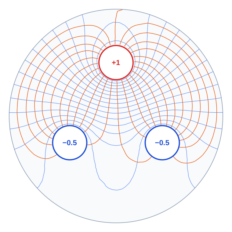
Consider an illustrative configuration of three conductors — “phases” — each kept at its own voltage $V_1, V_2, V_3$. The conductors impose a Dirichlet condition on their boundaries, $V|_{\partial\Omega_k}$ $= V_k$; the outer boundary of the computational domain is assumed insulated, which corresponds to the homogeneous Neumann condition $\partial V / \partial n$ $= 0$. The presence of at least one conductor makes the finite-element system non-degenerate, and it is solved by the same preconditioned conjugate gradient method.

The computed field picture is shown in figure Field of three conductors: the equipotentials and the field lines form a mutually orthogonal grid; the field lines leave the positive phase and terminate on the negative ones.