Triangulation

In the two-dimensional case the simplex is a triangle, so for a given set of points we must build a family of triangles that covers the domain completely and has no internal intersections. Additionally we require the resulting mesh to satisfy the Delaunay condition: the circumscribed circle of each triangle must contain no other vertices of the triangulation. For a non-degenerate point set without prescribed edges, such a triangulation maximizes the minimum angle. Thus the Delaunay condition helps reduce the number of badly elongated triangles, while the stability of the subsequent finite-element computations also depends on the input geometry quality, point density and correct handling of constraints.

Building a Delaunay mesh by hand is trickier than it seems: the computational domain is often a square or an annulus, whose boundaries produce degenerate configurations on which naive floating-point computations fail (see below). The low-level construction is therefore entrusted to the mature CGAL library with exact geometric predicates, with a data-preparation and validation pipeline implemented on top. The project's own implementation of the classical divide-and-conquer scheme, with which it all started, has been moved to the appendix “Triangulation by divide and conquer”.

Geometric predicates

Almost every geometric decision in the algorithm reduces to two sign predicates.

Position of a point relative to an edge. For a directed edge with endpoints $p_1$ $=(x_1,y_1)$, $p_2$ $=(x_2,y_2)$ and a point $p_3$ $=(x_3,y_3)$, the sign of the expression

determines whether $p_3$ lies to the left, to the right, or exactly on the line $p_1 p_2$. The same predicate is used when building the convex hull and when controlling triangle orientation.

Testing the Delaunay condition. For a triangle with vertices $p_1, p_2, p_3$ listed counter-clockwise and a query point $p_0$ $=(x_0,y_0)$, the condition is conveniently written via the sign of the determinant

If condition (4.2)$\displaystyle \det \begin{pmatrix} x_1 & y_1 & x_1^2 + y_1^2 & 1 \\ x_2 & y_2 & x_2^2 + y_2^2 & 1 \\ x_3 & y_3 & x_3^2 + y_3^2 & 1 \\ x_0 & y_0 & x_0^2 + y_0^2 & 1 \end{pmatrix}$ $\displaystyle \leq 0$ holds, the point $p_0$ lies outside the circumscribed circle or on its boundary; otherwise it is inside, and the pair of adjacent triangles must be restructured. With clockwise vertex order the sign of the determinant flips, so triangle orientation is controlled by predicate (4.1)$\displaystyle \operatorname{orient}(p_1,p_2,p_3)$ $\displaystyle = (x_2 - x_1)(y_3 - y_1)$ $\displaystyle - (y_2 - y_1)(x_3 - x_1)$.

Robustness on degenerate input

Predicates (4.1)$\displaystyle \operatorname{orient}(p_1,p_2,p_3)$ $\displaystyle = (x_2 - x_1)(y_3 - y_1)$ $\displaystyle - (y_2 - y_1)(x_3 - x_1)$ and (4.2)$\displaystyle \det \begin{pmatrix} x_1 & y_1 & x_1^2 + y_1^2 & 1 \\ x_2 & y_2 & x_2^2 + y_2^2 & 1 \\ x_3 & y_3 & x_3^2 + y_3^2 & 1 \\ x_0 & y_0 & x_0^2 + y_0^2 & 1 \end{pmatrix}$ $\displaystyle \leq 0$ are signs of determinants. On inputs in general position their value differs noticeably from zero, and ordinary double-precision arithmetic yields the correct sign. But a square computational domain produces two unpleasant cases:

• collinearity — many boundary points lie exactly on one vertical or horizontal line, and predicate (4.1)$\displaystyle \operatorname{orient}(p_1,p_2,p_3)$ $\displaystyle = (x_2 - x_1)(y_3 - y_1)$ $\displaystyle - (y_2 - y_1)(x_3 - x_1)$ evaluates to exact zero;
• cocircularity — the four corners of any cell of a regular grid lie on one circle, and determinant (4.2)$\displaystyle \det \begin{pmatrix} x_1 & y_1 & x_1^2 + y_1^2 & 1 \\ x_2 & y_2 & x_2^2 + y_2^2 & 1 \\ x_3 & y_3 & x_3^2 + y_3^2 & 1 \\ x_0 & y_0 & x_0^2 + y_0^2 & 1 \end{pmatrix}$ $\displaystyle \leq 0$ is also exactly zero.

The trouble is that when such a “zero” determinant is computed in floating-point arithmetic, rounding errors accumulate, and instead of zero we get a tiny number of arbitrary sign — noise. Different parts of the algorithm, having received contradictory answers for the same triple of points, start building an inconsistent mesh: flat (zero-area) triangles appear along the boundary and the Delaunay condition is violated.

The solution is to compute the sign of the predicate exactly. The library we use evaluates the determinants with filtered arithmetic: a fast preliminary computation with a guaranteed error bound, and in doubtful (near-zero) cases an exact re-evaluation. As a result the sign is never wrong, and a true zero is recognized as zero. Importantly, only the predicates need exactness: the algorithm constructs no new points — the mesh vertices are exactly the input points — so exact construction arithmetic is not required and the coordinates remain plain double-precision numbers. This compromise costs almost nothing in speed.

Constrained triangulation

In practice, besides the points themselves we must honour user-specified edges — the boundaries of the computational domain and the contours of holes. Such edges must be present in the final mesh and must not be destroyed by local restructurings. This problem is known as constrained Delaunay triangulation: near a constraint edge the Delaunay condition may legitimately be violated, but in return the mesh is guaranteed to follow the prescribed contours. The edge-insertion operation itself is described below in the implementation section, and in full detail in the appendix.

Meshing the computational domain

The full pipeline that meshes a domain with a boundary and holes consists of six steps.

1. The contours — the outer one and the hole contours — are subdivided into segments no longer than the target step $\sqrt{S/n}$, where $S$ is the domain area and $n$ is the number of interior points; this matches the boundary point density to the interior density and reduces the risk of elongated triangles along the boundary.
2. $n$ random points are generated inside the domain (outside the holes) by rejection sampling, optionally with a prescribed minimum distance between them.
3. The interior points are inserted one by one into an empty triangulation, followed by the boundary points of all contours.
4. Every segment of every contour is forcibly inserted into the mesh as a constraint edge.
5. The resulting triangulation — it still covers the whole convex hull — is validated; on any defect the construction aborts with an error.
6. Triangles whose centroid lies outside the domain (inside a hole or beyond the outer contour) are discarded — what remains is the mesh of the computational domain proper.

The validation in step five is a safety net comprising four checks:

• vertex completeness — every input point is present in the mesh as a vertex, and the mesh contains no extraneous vertices;
• triangle count — it must equal the value $T$ $= 2N$ $- 2$ $- h$ that follows from Euler's formula, where $N$ is the number of vertices and $h$ is the number of vertices on the convex hull;
• non-intersection — no two triangles intersect across edge interiors;
• Delaunay condition — checked for pairs of triangles whose shared side is not a constraint edge; near constraints the Delaunay condition may legitimately be violated.

Storing the triangulation

The finished triangulation is stored not as a mere list of triangles but as a structure that maps every edge to its adjacent triangles. Through a shared edge one can always quickly find the pair of triangles potentially violating the Delaunay condition — this is what flip operations use. The same structure yields the mesh boundary (edges belonging to a single triangle): before the holes are cut out, that is the convex hull. The output is a set of triangular simplices from which the local stiffness matrices are later built and the global finite-element system is assembled.

Implementation: the CGAL library

CGAL (Computational Geometry Algorithms Library) is an open-source C++ computational-geometry library and the de facto standard in the field. We use its classes Delaunay_triangulation_2 (plain Delaunay triangulation) and Constrained_Delaunay_triangulation_2 (constrained triangulation) with the Exact_predicates_inexact_constructions_kernel. The staged pipeline described above, the constraint insertion and the step-five checks are implemented on top of it.

CGAL builds the mesh incrementally — points are inserted one by one into an existing triangulation.

• Instead of an auxiliary “super-triangle”, which would have to be sized and later deleted, it uses an infinite vertex: the convex hull of the current mesh is closed off by fictitious triangles whose third vertex is a formal “point at infinity”.
• Each next point is first located by walking the mesh: starting from some triangle, the algorithm steps from neighbour to neighbour towards the point, guided by orientation predicate (4.1)$\displaystyle \operatorname{orient}(p_1,p_2,p_3)$ $\displaystyle = (x_2 - x_1)(y_3 - y_1)$ $\displaystyle - (y_2 - y_1)(x_3 - x_1)$.
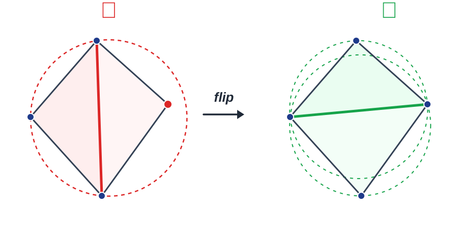
• The located triangle is split by the inserted point into three (a point on an edge splits the two adjacent triangles into four), after which the Delaunay condition is restored by a cascade of flips spreading from the new vertex: if by predicate (4.2)$\displaystyle \det \begin{pmatrix} x_1 & y_1 & x_1^2 + y_1^2 & 1 \\ x_2 & y_2 & x_2^2 + y_2^2 & 1 \\ x_3 & y_3 & x_3^2 + y_3^2 & 1 \\ x_0 & y_0 & x_0^2 + y_0^2 & 1 \end{pmatrix}$ $\displaystyle \leq 0$ the fourth vertex of the neighbouring triangle falls inside the circumscribed circle, the common diagonal of the quadrilateral is replaced by the opposite one (figure Diagonal swap).

A constraint edge is inserted into the finished mesh by a separate operation: all triangles crossed by the segment are removed, the resulting cavity is split by the segment into two chains of vertices, and each chain is re-triangulated; in subsequent restructurings, flipping across the constraint edge is forbidden. Since by insertion time both endpoints of every segment are already mesh vertices and the contours do not intersect, no new (Steiner) points appear. A detailed walkthrough of this operation is given in the appendix.

The chosen kernel combines exact predicates with inexact constructions. Predicates are evaluated with filtering: interval arithmetic with a guaranteed error bound first, and only when the interval straddles zero — an exact re-evaluation in multiprecision arithmetic. This is what ensures that the collinear and cocircular configurations of the square are handled correctly. Constructions, in turn, stay plain doubles: the algorithm creates no new points, so every vertex of the final mesh maps back losslessly to an input point. With a random insertion order — which our random point generator provides — the expected construction cost is $O(n \log n)$.

Examples

All meshes below are real outputs of the described pipeline (the triangulate utility of the computational core), drawn without any retouching.

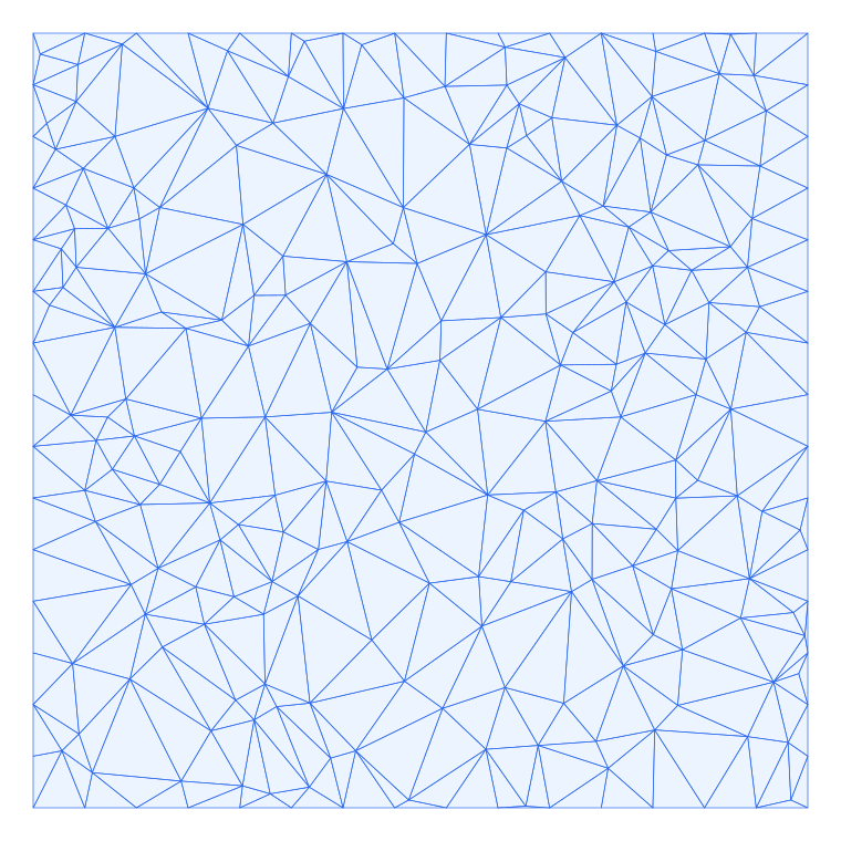
The figure “Square” shows the triangulation of the unit square with $n$ $= 200$ interior points: after the boundary is subdivided with step $\sqrt{S/n}$, the mesh contains 260 vertices and 458 triangles. The square's boundary consists of dozens of exactly collinear points — the very degenerate input on which floating-point arithmetic without exact predicates falls apart; here the mesh is correct along the entire boundary, with no flat triangles.

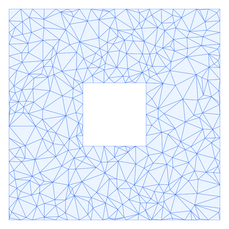
The figure “Square with a hole” demonstrates constraint edges at work: a square hole is cut out of the square, and both contours are inserted as constraints ($n$ $= 300$; 396 vertices, 696 triangles). The mesh follows the hole contour exactly and does not enter it — triangles whose centroid landed inside the hole were discarded at the final pipeline step.

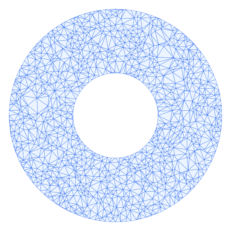
Finally, the figure “Annulus” shows the triangulation of an annulus (outer radius 1, inner radius 0.4) with $n$ $= 1000$: the final mesh contains 1192 vertices and 2192 triangles. Both contours are approximated by polygons (128 and 64 vertices) and inserted as constraint edges, so the mesh follows the prescribed polygonal boundary of the domain, while the interior points produce a nearly uniform Delaunay mesh.