When solving boundary value problems by separation of variables, the partial differential equation splits into ordinary differential equations in each coordinate. Depending on the coordinate system and the geometry of the domain, these equations lead to different families of orthogonal functions.
The Bessel functions of the first kind . They arise when separating variables in polar and cylindrical coordinates: the radial part of the Helmholtz equation reduces to the Bessel equation
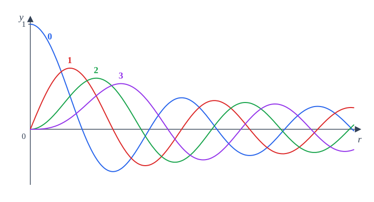
The graphs of the first orders are shown in figure (B.1).
Fig. B.1. The Bessel functions of the first kind of orders .
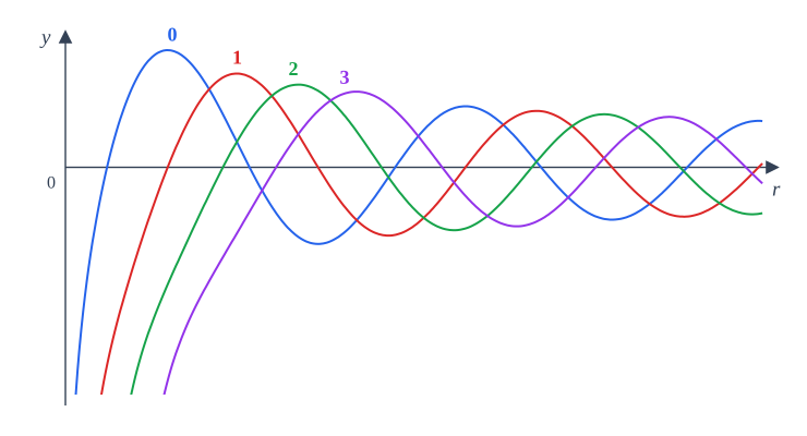
The Neumann functions (Bessel functions of the second kind). They arise as the second linearly independent solution of the same Bessel equation. Unlike , they grow unboundedly in absolute value near the axis: for . Therefore, in problems where the domain includes the axis , they are discarded by the requirement that the solution be bounded, but in annular domains (not containing the axis) they enter the solution on a par with . The graphs of the first orders are shown in figure (B.2).
Fig. B.2. The Neumann functions of orders .
The spherical Bessel functions . They appear in the radial part of the Helmholtz equation in spherical coordinates
The substitution reduces it to the Bessel equation of half-integer order, so the solutions are expressed in terms of ordinary Bessel functions
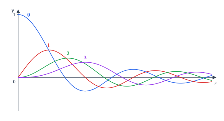
As in the cylindrical case, oscillate with decreasing amplitude; their graphs are shown in figure (B.3).
Fig. B.3. The spherical Bessel functions of orders .
The Legendre polynomials . They arise from the angular (polar) part of the Helmholtz equation in spherical coordinates. After the substitution and for the equation takes the form of the Legendre equation
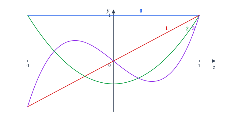
whose solutions bounded on the interval are the Legendre polynomials of degree . They form an orthogonal basis on ; the first few are shown in figure (B.4).
Fig. B.4. The Legendre polynomials of degrees .
The associated Legendre functions . If in the polar part , the Legendre equation generalizes to the associated equation
whose solutions are the associated Legendre functions , expressed in terms of the Legendre polynomials
For they turn into the Legendre polynomials , and together with the azimuthal factor or form the angular part of the eigenfunction.