Test functions

The function that describes the behaviour on a simplex is called a test function — probably because in the early days of the method, given how weak computing hardware was, one had to try out and tune functions that would approximate the solution. There is a vast number of test functions — one can even use trigonometric ones — but in practice polynomial functions became the common choice, which hints at expanding the solution in a Taylor series, by analogy with the expansion in a Fourier series, with the sole difference that we carry out the Taylor expansion not over the whole geometry, but only on the simplices, which lets us use the simplest possible polynomials. As a rule, polynomials of degree 3 were chosen, with 9–10 coefficients, and this required adding extra points to the simplex in order to determine those coefficients, which led to 9–10 systems of linear equations on each simplex; but they had to be solved only once, which, computationally, is not a problem even by the standards of that time. This is, of course, a sound approach, but I decided to “try” building the solution with the simplest possible polynomials, namely polynomials of the form:

υh(x,y,z)\displaystyle \upsilon_h(x,y,z) =i=1nqiϕi(x,y,z),\displaystyle = \sum_{i=1}^{n} q_i \cdot \phi_i(x, y, z),
(5.5)

where nn is the number of nodes, qiq_i are the coefficients, ϕi(x,y,z)\phi_i(x, y, z) are the so-called “hat” functions, which equal 1 at a node of the simplex and 0 at the remaining nodes of the geometry; and it is precisely because the “hat” functions are polynomials that the test functions, too, will be polynomials.

ϕi(x,y,z)\displaystyle \phi_i(x,y,z) =ai\displaystyle = a_{i} +bix\displaystyle + b_{i} \cdot x +ciy\displaystyle + c_{i} \cdot y +diz,\displaystyle + d_{i} \cdot z,
(5.6)

where ii is the node index, not a power, ai,bi,ci,dia_{i}, b_{i}, c_{i}, d_{i} are the coefficients that depend on the geometry of the particular node ii on the simplex. Once the geometry has been partitioned into simplices, they will need to be computed once for each node of the simplex. I wrote the “hat” function for a three-dimensional coordinate system, but further on we will work with the two-dimensional or one-dimensional case in the same way.

Let us discuss the “hat” functions in more detail and start with the one-dimensional case.
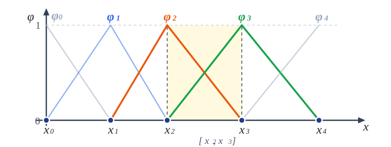
One-dimensional linear hat functions
Fig. 5.4. “Hat” functions for segment simplices.

In figure “Hat” functions for segment simplices five “hat” functions are shown — ϕ0,,ϕ4\phi_0, …, \phi_4 and four simplices: in total, for one-dimensional space, over nn points there are nn “hat” functions and nn 1- 1 simplices, respectively. At the ends, at the nodes x0x_0 and x4x_4, the functions take the form of half-“hats”. Let us take ii =3= 3; then the simplex between the points xi1x_{i-1} and xix_i (in the figure it is highlighted with a fill and bounded by dashed lines) is defined as follows: υi1(x)\upsilon_{i-1}(x) =qi1ϕi1(x)= q_{i-1} \cdot \phi_{i-1}(x) +qiϕi(x)+ q_i \cdot \phi_i(x), since the remaining “hat” functions have no effect on it because they take the value zero on the interval (xi1,xi)(x_{i-1}, x_i). The function ϕi1(x)\phi_{i-1}(x) passes through the points (xi1,1)(x_{i-1}, 1) and (xi,0)(x_i, 0), and the function ϕi(x)\phi_i(x) through the points (xi1,0)(x_{i-1}, 0) and (xi,1)(x_i, 1). Then the following holds

{ai1+bi1xi1=1ai1+bi1xi=0{ai+bixi1=0ai+bixi=1\begin{cases} a_{i-1} + b_{i-1} \cdot x_{i-1} = 1\\ a_{i-1} + b_{i-1} \cdot x_i = 0 \end{cases} \begin{cases} a_{i} + b_{i} \cdot x_{i-1} = 0\\ a_{i} + b_{i} \cdot x_i = 1 \end{cases}
(5.7)

The solutions of the systems are, respectively

{ai1=xixi1xibi1=1xi1xi{ai=xi1xi1xibi=1xi1xi\begin{cases} a_{i-1} = \frac{\displaystyle -x_i}{\displaystyle x_{i-1} - x_i}\\ b_{i-1} = \frac{\displaystyle 1}{\displaystyle x_{i-1} - x_i} \end{cases} \begin{cases} a_{i} = \frac{\displaystyle x_{i-1}}{\displaystyle x_{i-1} - x_i}\\ b_{i} = \frac{\displaystyle -1}{\displaystyle x_{i-1} - x_i} \end{cases}
(5.8)

If for one-dimensional simplices the “hat” functions look like lines in the plane, then for two-dimensional simplices they become surfaces in three-dimensional space.

Fig. 5.5. “Hat” functions for triangle simplices.

We took all three vertices of the triangle t2t_2 from figure Triangle simplices and built three pyramids whose apexes are the vertices of the original triangle “raised” by 1, while the bases of the pyramids are the polygons from the same figure that contain the triangle’s vertices inside them. Since the triangle under study is t2t_2 and we intend to write the test function for it, let us discard the extra parts and redraw the figure, keeping only the planes that project onto the triangle.

Fig. 5.6. Parts of the “hat” functions for a triangle simplex.

In figure Parts of the “hat” functions for a triangle simplex for two-dimensional space, just as for the one-dimensional case, to each of the nn mesh nodes there corresponds exactly one “hat” function, so there are nn of them in total; the number of triangle simplices, however, depends on the particular triangulation. Note also that within a single triangle exactly three “hat” functions are nonzero — one for each of its vertices. Let us denote the vertices of the simplex by (xi,yi),(xi+1,yi+1),(xi+2,yi+2)(x_i, y_i), (x_{i+1}, y_{i+1}), (x_{i+2}, y_{i+2}). As a result, the test function takes the form υi(x,y)\upsilon_i(x, y) =qiϕi(x,y)= q_i \cdot \phi_i(x, y) +qi+1ϕi+1(x,y)+ q_{i+1} \cdot \phi_{i+1}(x, y) +qi+2ϕi+2(x,y)+ q_{i+2} \cdot \phi_{i+2}(x, y). To determine the constants ai,bi,cia_{i},b_{i},c_{i}, ai+1,bi+1,ci+1a_{i+1},b_{i+1},c_{i+1}, ai+2,bi+2,ci+2a_{i+2},b_{i+2},c_{i+2} let us take into account that the coordinate zz is nonzero only at the apexes of the pyramids; as a result, we obtain three systems of equations

{ai+bixi+ciyi=1ai+bixi+1+ciyi+1=0ai+bixi+2+ciyi+2=0{ai+1+bi+1xi+ci+1yi=0ai+1+bi+1xi+1+ci+1yi+1=1ai+1+bi+1xi+2+ci+1yi+2=0{ai+2+bi+2xi+ci+2yi=0ai+2+bi+2xi+1+ci+2yi+1=0ai+2+bi+2xi+2+ci+2yi+2=1\begin{cases} a_{i} + b_{i} \cdot x_i + c_{i} \cdot y_i = 1\\ a_{i} + b_{i} \cdot x_{i+1} + c_{i} \cdot y_{i+1} = 0\\ a_{i} + b_{i} \cdot x_{i+2} + c_{i} \cdot y_{i+2} = 0 \end{cases} \begin{cases} a_{i+1} + b_{i+1} \cdot x_i + c_{i+1} \cdot y_i = 0\\ a_{i+1} + b_{i+1} \cdot x_{i+1} + c_{i+1} \cdot y_{i+1} = 1\\ a_{i+1} + b_{i+1} \cdot x_{i+2} + c_{i+1} \cdot y_{i+2} = 0 \end{cases} \begin{cases} a_{i+2} + b_{i+2} \cdot x_i + c_{i+2} \cdot y_i = 0\\ a_{i+2} + b_{i+2} \cdot x_{i+1} + c_{i+2} \cdot y_{i+1} = 0\\ a_{i+2} + b_{i+2} \cdot x_{i+2} + c_{i+2} \cdot y_{i+2} = 1 \end{cases}
(5.9)

The solutions of the equations are, respectively

{ai=(xi+1yi+2xi+2yi+1)/detbi=(yi+1yi+2)/detci=(xi+1+xi+2)/det{ai+1=(xiyi+2+xi+2yi)/detbi+1=(yi+yi+2)/detci+1=(xixi+2)/det{ai+2=(xiyi+1xi+1yi)/detbi+2=(yiyi+1)/detci+2=(xi+xi+1)/det\begin{cases} a_{i} = (x_{i+1} \cdot y_{i+2} - x_{i+2} \cdot y_{i+1}) / \det\\ b_{i} = (y_{i+1} - y_{i+2}) / \det\\ c_{i} = (-x_{i+1} + x_{i+2}) / \det \end{cases} \begin{cases} a_{i+1} = ( - x_i \cdot y_{i+2} + x_{i+2} \cdot y_i) / \det\\ b_{i+1} = (-y_i + y_{i+2}) / \det\\ c_{i+1} = (x_i - x_{i+2}) / \det \end{cases} \begin{cases} a_{i+2} = (x_i \cdot y_{i+1} - x_{i+1} \cdot y_i) / \det\\ b_{i+2} = (y_i - y_{i+1}) / \det\\ c_{i+2} = (-x_i + x_{i+1}) / \det \end{cases}
(5.10)

where det\det =xiyi+1= x_i \cdot y_{i+1} xiyi+2- x_i \cdot y_{i+2} xi+1yi- x_{i+1} \cdot y_i +xi+1yi+2+ x_{i+1} \cdot y_{i+2} +xi+2yi+ x_{i+2} \cdot y_i xi+2yi+1- x_{i+2} \cdot y_{i+1} is the determinant of the matrix.

The difficulty of working with a three-dimensional coordinate system is that the solution, like the “hat” functions, is hard to visualise, so we will make do with formulas alone. In general, this guide places its main emphasis on two-dimensional boundary-value problems, since, unlike the one-dimensional ones, they are not trivial and at the same time visualise well. So, in three-dimensional space a tetrahedron serves as the base of a four-dimensional pentachoron-“hat”. By analogy with the formulas above, we venture to assume that the “hat” function will take the value 1 at one of the vertices of the tetrahedron — raised into four-dimensional space perpendicular to the base — and be zero at the remaining nodes of the tetrahedralization; the test function then takes the form υh(x,y,z)\upsilon_h(x, y, z) =q1ϕ1(x,y,z)= q_1 \cdot \phi_1(x, y, z) +q2ϕ2(x,y,z)+ q_2 \cdot \phi_2(x, y, z) +q3ϕ3(x,y,z)+ q_3 \cdot \phi_3(x, y, z) +q4ϕ4(x,y,z)+ q_4 \cdot \phi_4(x, y, z). To determine the constants ai,bi,ci,dia_{i},b_{i},c_{i},d_{i}, ai+1,bi+1,ci+1,di+1a_{i+1},b_{i+1},c_{i+1},d_{i+1}, ai+2,bi+2,ci+2,di+2a_{i+2},b_{i+2},c_{i+2},d_{i+2}, ai+3,bi+3,ci+3,di+3a_{i+3},b_{i+3},c_{i+3},d_{i+3} let us take into account that the coordinate μ\mu of the fourth dimension is nonzero only at the apexes of the pentachora; as a result, we obtain four systems of equations

{ai+bixi+ciyi+dizi=1ai+bixi+1+ciyi+1+dizi+1=0ai+bixi+2+ciyi+2+dizi+2=0ai+bixi+3+ciyi+3+dizi+3=0{ai+1+bi+1xi+ci+1yi+di+1zi=0ai+1+bi+1xi+1+ci+1yi+1+di+1zi+1=1ai+1+bi+1xi+2+ci+1yi+2+di+1zi+2=0ai+1+bi+1xi+3+ci+1yi+3+di+1zi+3=0{ai+2+bi+2xi+ci+2yi+di+2zi=0ai+2+bi+2xi+1+ci+2yi+1+di+2zi+1=0ai+2+bi+2xi+2+ci+2yi+2+di+2zi+2=1ai+2+bi+2xi+3+ci+2yi+3+di+2zi+3=0{ai+3+bi+3xi+ci+3yi+di+3zi=0ai+3+bi+3xi+1+ci+3yi+1+di+3zi+1=0ai+3+bi+3xi+2+ci+3yi+2+di+3zi+2=0ai+3+bi+3xi+3+ci+3yi+3+di+3zi+3=1\begin{cases} a_{i} + b_{i} \cdot x_i + c_{i} \cdot y_i + d_{i} \cdot z_i = 1\\ a_{i} + b_{i} \cdot x_{i+1} + c_{i} \cdot y_{i+1} + d_{i} \cdot z_{i+1} = 0\\ a_{i} + b_{i} \cdot x_{i+2} + c_{i} \cdot y_{i+2} + d_{i} \cdot z_{i+2} = 0\\ a_{i} + b_{i} \cdot x_{i+3} + c_{i} \cdot y_{i+3} + d_{i} \cdot z_{i+3} = 0 \end{cases} \begin{cases} a_{i+1} + b_{i+1} \cdot x_i + c_{i+1} \cdot y_i + d_{i+1} \cdot z_i = 0\\ a_{i+1} + b_{i+1} \cdot x_{i+1} + c_{i+1} \cdot y_{i+1} + d_{i+1} \cdot z_{i+1} = 1\\ a_{i+1} + b_{i+1} \cdot x_{i+2} + c_{i+1} \cdot y_{i+2} + d_{i+1} \cdot z_{i+2} = 0\\ a_{i+1} + b_{i+1} \cdot x_{i+3} + c_{i+1} \cdot y_{i+3} + d_{i+1} \cdot z_{i+3} = 0 \end{cases} \begin{cases} a_{i+2} + b_{i+2} \cdot x_i + c_{i+2} \cdot y_i + d_{i+2} \cdot z_i = 0\\ a_{i+2} + b_{i+2} \cdot x_{i+1} + c_{i+2} \cdot y_{i+1} + d_{i+2} \cdot z_{i+1} = 0\\ a_{i+2} + b_{i+2} \cdot x_{i+2} + c_{i+2} \cdot y_{i+2} + d_{i+2} \cdot z_{i+2} = 1\\ a_{i+2} + b_{i+2} \cdot x_{i+3} + c_{i+2} \cdot y_{i+3} + d_{i+2} \cdot z_{i+3} = 0 \end{cases} \begin{cases} a_{i+3} + b_{i+3} \cdot x_i + c_{i+3} \cdot y_i + d_{i+3} \cdot z_i = 0\\ a_{i+3} + b_{i+3} \cdot x_{i+1} + c_{i+3} \cdot y_{i+1} + d_{i+3} \cdot z_{i+1} = 0\\ a_{i+3} + b_{i+3} \cdot x_{i+2} + c_{i+3} \cdot y_{i+2} + d_{i+3} \cdot z_{i+2} = 0\\ a_{i+3} + b_{i+3} \cdot x_{i+3} + c_{i+3} \cdot y_{i+3} + d_{i+3} \cdot z_{i+3} = 1 \end{cases}
(5.11)

The solutions of the equations are, respectively

{ai=(xi+1yi+2zi+3+xi+1yi+3zi+2+xi+2yi+1zi+3xi+2yi+3zi+1xi+3yi+1zi+2+xi+3yi+2zi+1)/detbi=(yi+1zi+2yi+1zi+3yi+2zi+1+yi+2zi+3+yi+3zi+1yi+3zi+2)/detci=(xi+1zi+2+xi+1zi+3+xi+2zi+1xi+2zi+3xi+3zi+1+xi+3zi+2)/detdi=(xi+1yi+2xi+1yi+3xi+2yi+1+xi+2yi+3+xi+3yi+1xi+3yi+2)/det{ai+1=(xiyi+2zi+3xiyi+3zi+2xi+2yizi+3+xi+2yi+3zi+xi+3yizi+2xi+3yi+2zi)/detbi+1=(yizi+2+yizi+3+yi+2ziyi+2zi+3yi+3zi+yi+3zi+2)/detci+1=(xizi+2xizi+3xi+2zi+xi+2zi+3+xi+3zixi+3zi+2)/detdi+1=(xiyi+2+xiyi+3+xi+2yixi+2yi+3xi+3yi+xi+3yi+2)/det{ai+2=(xiyi+1zi+3+xiyi+3zi+1+xi+1yizi+3xi+1yi+3zixi+3yizi+1+xi+3yi+1zi)/detbi+2=(yizi+1yizi+3yi+1zi+yi+1zi+3+yi+3ziyi+3zi+1)/detci+2=(xizi+1+xizi+3+xi+1zixi+1zi+3xi+3zi+xi+3zi+1)/detdi+2=(xiyi+1xiyi+3xi+1yi+xi+1yi+3+xi+3yixi+3yi+1)/det{ai+3=(xiyi+1zi+2xiyi+2zi+1xi+1yizi+2+xi+1yi+2zi+xi+2yizi+1xi+2yi+1zi)/detbi+3=(yizi+1+yizi+2+yi+1ziyi+1zi+2yi+2zi+yi+2zi+1)/detci+3=(xizi+1xizi+2xi+1zi+xi+1zi+2+xi+2zixi+2zi+1)/detdi+3=(xiyi+1+xiyi+2+xi+1yixi+1yi+2xi+2yi+xi+2yi+1)/det\begin{cases} a_{i} = (-x_{i+1} \cdot y_{i+2} \cdot z_{i+3} + x_{i+1} \cdot y_{i+3} \cdot z_{i+2} + x_{i+2} \cdot y_{i+1} \cdot z_{i+3} - x_{i+2} \cdot y_{i+3} \cdot z_{i+1} \\- x_{i+3} \cdot y_{i+1} \cdot z_{i+2} + x_{i+3} \cdot y_{i+2} \cdot z_{i+1}) / \det\\ b_{i} = (y_{i+1} z_{i+2} - y_{i+1} z_{i+3} - y_{i+2} z_{i+1} + y_{i+2} z_{i+3} + y_{i+3} z_{i+1} - y_{i+3} z_{i+2}) / \det\\ c_{i} = (-x_{i+1} z_{i+2} + x_{i+1} z_{i+3} + x_{i+2} z_{i+1} - x_{i+2} z_{i+3} - x_{i+3} z_{i+1} + x_{i+3} z_{i+2}) / \det\\ d_{i} = (x_{i+1} y_{i+2} - x_{i+1} y_{i+3} - x_{i+2} y_{i+1} + x_{i+2} y_{i+3} + x_{i+3} y_{i+1} - x_{i+3} y_{i+2}) / \det \end{cases} \begin{cases} a_{i+1} = (x_i \cdot y_{i+2} \cdot z_{i+3} - x_i \cdot y_{i+3} \cdot z_{i+2} - x_{i+2} \cdot y_i \cdot z_{i+3} + x_{i+2} \cdot y_{i+3} \cdot z_i \\+ x_{i+3} \cdot y_i \cdot z_{i+2} - x_{i+3} \cdot y_{i+2} \cdot z_i) / \det\\ b_{i+1} = (-y_i z_{i+2} + y_i z_{i+3} + y_{i+2} z_i - y_{i+2} z_{i+3} - y_{i+3} z_i + y_{i+3} z_{i+2}) / \det\\ c_{i+1} = (x_i z_{i+2} - x_i z_{i+3} - x_{i+2} z_i + x_{i+2} z_{i+3} + x_{i+3} z_i - x_{i+3} z_{i+2}) / \det\\ d_{i+1} = (-x_i y_{i+2} + x_i y_{i+3} + x_{i+2} y_i - x_{i+2} y_{i+3} - x_{i+3} y_i + x_{i+3} y_{i+2}) / \det \end{cases} \begin{cases} a_{i+2} = (-x_i \cdot y_{i+1} \cdot z_{i+3} + x_i \cdot y_{i+3} \cdot z_{i+1} + x_{i+1} \cdot y_i \cdot z_{i+3} - x_{i+1} \cdot y_{i+3} \cdot z_i \\- x_{i+3} \cdot y_i \cdot z_{i+1} + x_{i+3} \cdot y_{i+1} \cdot z_i) / \det\\ b_{i+2} = (y_i z_{i+1} - y_i z_{i+3} - y_{i+1} z_i + y_{i+1} z_{i+3} + y_{i+3} z_i - y_{i+3} z_{i+1}) / \det\\ c_{i+2} = (-x_i z_{i+1} + x_i z_{i+3} + x_{i+1} z_i - x_{i+1} z_{i+3} - x_{i+3} z_i + x_{i+3} z_{i+1}) / \det\\ d_{i+2} = (x_i y_{i+1} - x_i y_{i+3} - x_{i+1} y_i + x_{i+1} y_{i+3} + x_{i+3} y_i - x_{i+3} y_{i+1}) / \det \end{cases} \begin{cases} a_{i+3} = (x_i \cdot y_{i+1} \cdot z_{i+2} - x_i \cdot y_{i+2} \cdot z_{i+1} - x_{i+1} \cdot y_i \cdot z_{i+2} + x_{i+1} \cdot y_{i+2} \cdot z_i \\+ x_{i+2} \cdot y_i \cdot z_{i+1} - x_{i+2} \cdot y_{i+1} \cdot z_i) / \det\\ b_{i+3} = (-y_i z_{i+1} + y_i z_{i+2} + y_{i+1} z_i - y_{i+1} z_{i+2} - y_{i+2} z_i + y_{i+2} z_{i+1}) / \det\\ c_{i+3} = (x_i z_{i+1} - x_i z_{i+2} - x_{i+1} z_i + x_{i+1} z_{i+2} + x_{i+2} z_i - x_{i+2} z_{i+1}) / \det\\ d_{i+3} = (-x_i y_{i+1} + x_i y_{i+2} + x_{i+1} y_i - x_{i+1} y_{i+2} - x_{i+2} y_i + x_{i+2} y_{i+1}) / \det \end{cases}
(5.12)

where the determinant of the matrix is:

det\displaystyle \det =xiyi+1zi+2\displaystyle ={} x_i \cdot y_{i+1} \cdot z_{i+2} xiyi+1zi+3\displaystyle - x_i \cdot y_{i+1} \cdot z_{i+3} xiyi+2zi+1\displaystyle - x_i \cdot y_{i+2} \cdot z_{i+1} +xiyi+2zi+3\displaystyle + x_i \cdot y_{i+2} \cdot z_{i+3} +xiyi+3zi+1\displaystyle + x_i \cdot y_{i+3} \cdot z_{i+1} xiyi+3zi+2\displaystyle - x_i \cdot y_{i+3} \cdot z_{i+2} xi+1yizi+2\displaystyle - x_{i+1} \cdot y_i \cdot z_{i+2} +xi+1yizi+3\displaystyle + x_{i+1} \cdot y_i \cdot z_{i+3} +xi+1yi+2zi\displaystyle + x_{i+1} \cdot y_{i+2} \cdot z_i xi+1yi+2zi+3\displaystyle - x_{i+1} \cdot y_{i+2} \cdot z_{i+3} xi+1yi+3zi\displaystyle - x_{i+1} \cdot y_{i+3} \cdot z_i +xi+1yi+3zi+2\displaystyle + x_{i+1} \cdot y_{i+3} \cdot z_{i+2} +xi+2yizi+1\displaystyle + x_{i+2} \cdot y_i \cdot z_{i+1} xi+2yizi+3\displaystyle - x_{i+2} \cdot y_i \cdot z_{i+3} xi+2yi+1zi\displaystyle - x_{i+2} \cdot y_{i+1} \cdot z_i +xi+2yi+1zi+3\displaystyle + x_{i+2} \cdot y_{i+1} \cdot z_{i+3} +xi+2yi+3zi\displaystyle + x_{i+2} \cdot y_{i+3} \cdot z_i xi+2yi+3zi+1\displaystyle - x_{i+2} \cdot y_{i+3} \cdot z_{i+1} xi+3yizi+1\displaystyle - x_{i+3} \cdot y_i \cdot z_{i+1} +xi+3yizi+2\displaystyle + x_{i+3} \cdot y_i \cdot z_{i+2} +xi+3yi+1zi\displaystyle + x_{i+3} \cdot y_{i+1} \cdot z_i xi+3yi+1zi+2\displaystyle - x_{i+3} \cdot y_{i+1} \cdot z_{i+2} xi+3yi+2zi\displaystyle - x_{i+3} \cdot y_{i+2} \cdot z_i +xi+3yi+2zi+1\displaystyle + x_{i+3} \cdot y_{i+2} \cdot z_{i+1}