This guide is devoted to thermal fields, which in general are nonstationary. Let us consider a small volume inside a body with boundary and outward unit normal (figure 1.1). The idea is simple: the amount of heat accumulated in the volume per unit time equals the heat inflow through its boundary plus the heat released inside by internal sources. This equation is called the energy balance equation and follows from the law of conservation of energy. Through the boundary there can be not only an inflow of heat but also an outflow, which is mathematically described as a negative inflow; similarly with internal sources, which can be consumers.
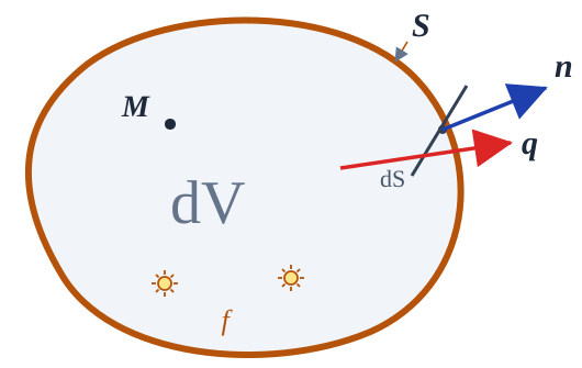
The formula for thermal energy is known , where is the thermal energy of the small volume , is the specific heat capacity , is the mass of the small volume , is the temperature . The mass of the small volume can be written in terms of the density and the volume itself : . Then the energy stored in this small volume equals . The rate of change of the thermal energy of the volume equals
Now let us describe the heat transfer. Fourier's law states that the heat flux density is proportional to the temperature gradient and directed against it — heat flows from hot regions to cold ones:
where is the thermal conductivity . The minus sign precisely reflects the fact that the flux is directed toward decreasing temperature.
Let us assemble the energy balance. The rate of change of the energy of the volume equals the heat inflow through the boundary (the inward flux is , since is the outward one) plus the power of the internal sources with volume density :
The surface integral is inconvenient — we get rid of it by the Ostrogradsky–Gauss theorem, turning the flux through the boundary into a volume integral of the divergence:
Substituting (1.4) into (1.3) and collecting everything under one integral, we obtain
The volume was chosen arbitrarily, and the integral over any such volume equals zero — hence the integrand itself equals zero. Substituting Fourier's law (1.2), we arrive at the equation in differential form:
It remains to use the assumption made above. The medium is homogeneous and isotropic, so the thermal conductivity is the same at all points and in all directions — it can be taken outside the divergence sign, and is the Laplace operator:
Dividing both sides by and denoting — the thermal diffusivity — and the reduced source density , we finally obtain the heat conduction equation:
where is the thermal diffusivity, is the Laplace operator, is the geometry, is time , is the sought solution — the temperature field , is the heat source density function inside the body .
Equation (1.8) is an inhomogeneous equation, since the right-hand side contains the heat source density function . The corresponding homogeneous equation has the form
The importance of the homogeneous equation will become apparent later, when we obtain the general solution by the Fourier method of separation of variables.
For the test problems we will consider the following coordinate systems and Laplace operators.
In the one-dimensional case the Cartesian coordinate system is used :
In the two-dimensional case the polar coordinate system is used :
In the three-dimensional case the spherical coordinate system is used :