The Nyquist–Shannon Sampling Theorem

Let us start with an utterly simple example, namely: imagine a sinusoid given by the formula

where $A$ is the amplitude, $f$ is the frequency, and the independent variable $t$ runs over the interval $[0,\, 1]$. On a graph such a sinusoid looks even more trivial.

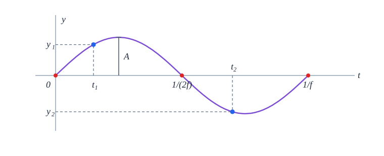
Any sinusoid given by formula (1) can be stored efficiently as just two numbers — the frequency and the amplitude; so to “compress” a sinusoid one has to read these two numbers off the graph of a single period. That is done by solving a system of equations

There are degenerate cases, of course: if both points land on zeros of the sinusoid, or sit symmetrically about its maximum, the equations become dependent and more than one sinusoid can pass through these two points. But on the whole it is all simple — and solving this system is not what matters to us. What matters is this: two points per period determine that very sinusoid uniquely.

An objection suggests itself here: how are you going to compute the frequency if you need two points inside a period, while the period itself is not yet known? A fair question with a simple answer: I measure at whatever rate the device has — say $f_s$ samples per second — take two neighbouring samples, solve the system (2) and obtain $f$. If the frequency that comes out is no more than half the measurement rate, that is $f$​${} \le f_s / 2$, then the measurement step did fit inside the period twice — so everything is computed correctly.

Naturally, a single sinusoid is of interest to nobody, so further on we shall talk about a linear combination of sinusoids — about the spectrum of a periodic — or periodized — signal. Periodicity is no restriction here: the theorem does not rely on it, and a period is needed only in order to speak of a set of harmonics. Say we observe a signal over a time $T$ — that very time is what we take for the period, and what the signal was doing before the observation began, or will be doing after, makes no difference to us.

First a few words about the Fourier series: what interests us is the passage from the time domain into the frequency domain and back. So let the signal $y(t)$ be periodic with period $T$, and let us denote the frequency of the $n$-th harmonic by $f_n$​${} = n / T$. The corresponding angular frequency is $\omega_n$​${} = 2 \pi f_n$. Passing into the frequency domain is two sets of coefficients, each computed by its own integral

and the signal is assembled back by summing all these harmonics

The constant term $a_0 / 2$ is the mean value of the signal. The frequencies $\omega_n$ sit on a grid with step $2 \pi / T$, so the spectrum of a periodic signal is simply a list of amplitudes $A_1, A_2, A_3, \ldots$.

As one can see, the more harmonics, the closer the signal is to the original one (about the Gibbs phenomenon we deliberately keep silent — it is not the subject of this article). It follows that digitizing a signal always loses some part of its spectrum. Sometimes that is even a good thing — this is how high-frequency noise is cut off and the signal is smoothed — but again, that is not my point. My point is that a band-limited signal is completely determined by its values taken at an angular sampling rate $\omega_s$​${} = 2 \pi f_s$​${} \ge 2 \omega_{\max}$, where $\omega_{\max}$ is the upper bound of its spectrum. What I have formulated above was formulated long ago by V. A. Kotelnikov — back in 1933. Independently of him the same theorem was obtained by others: Harry Nyquist pointed out the rate twice the signal’s highest frequency as early as 1928, and Claude Shannon published his own proof in 1949 and built it into the foundations of information theory — which is why in the English literature the theorem is usually called the Nyquist–Shannon sampling theorem.

To cover the question fully we ought to look at how the signal is reconstructed back from its spectrum. But first let us lay a little groundwork — write out the well-known trigonometric formulas.

Next we cannot do without the Dirichlet kernel — a closed formula for a sum of the form $\frac{1}{2}$​${} + \sum_{n=1}^{M} \cos(n x)$, so let us derive it right away. Multiply this sum by $2 \sin(x/2)$ and expand every term by the first formula of (5) — with $\alpha$​${} = (n + 1/2) x$ and $\beta$​${} = (n - 1/2) x$

the sum telescopes: the inner terms cancel pairwise, and the edge ones cancel against the $\sin(x/2)$ on the left. It remains to divide both sides by $2 \sin(x/2)$ — and that is the Dirichlet kernel

The groundwork is laid. Now let us take an arbitrary signal and its digitized version: the values are read off at the time instants $k \Delta t$ with a uniform step $\Delta t$.

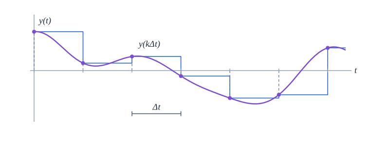
The measured signal is simply a set of numbers $y(k \Delta t)$, and it can be written through the Heaviside functions $\theta(t)$ — steps equal to zero for $t$​${} < 0$ and to one for $t$​${} \ge 0$: every sample holds its value until the next one, and the whole staircase turns out to be a linear combination of shifted steps

Now let us carry our staircase into the spectral domain, for which we compute the coefficients by formula (3). Take the cosine coefficient; inside the period there are $N$​${} = T / \Delta t$ steps — we number them from zero, from $k$​${} = 0$ to $k$​${} = N$​${} - 1$ — and the integral over the period falls apart into $N$ integrals over the steps, in each of which the value of the signal is constant and can be taken outside the integral

and by analogy for the sine coefficient we obtain

collapse the differences in (8) and (9) with the first two formulas of (5): the half-sum of the arguments here is the middle of the step, and the half-difference is one and the same for all $k$; let us denote

Note $\Lambda_n$ — this is the price of sampling. By the limit $\sin x / x$​${} \to 1$, the lower the frequency of the signal, or the smaller the interval $\Delta t$, the closer $\Lambda_n$ is to one. From (10) it is clear that the staircase gives the sums over the samples we need, multiplied by $\Lambda_n$ — so to obtain the sums themselves, (10) has to be divided by $\Lambda_n$. And now it is time to return from the frequency domain into the time domain.

A band-limited signal has no harmonics above $\omega_{\max}$, so the sum (4) breaks off: the last harmonic is the one with $\omega_n$​${} = \omega_{\max}$, that is $n$​${} = M$​${} = \omega_{\max} T / (2 \pi)$

substitute (10), divided by $\Lambda_n$, into it and swap the order of summation — first over the samples, then over the harmonics

and this sum of cosines we already know how to add up — it is the Dirichlet kernel (6) with $x$​${} = 2 \pi u / T$, where $u$​${} = t$​${} - t_k$ is the distance from the point $t$ to the middle of the step

it remains to let the period go to infinity — both the number of harmonics $M$ and the number of samples $N$​${} = T / \Delta t$ grow along with it. In the denominator $\sin(\pi u / T)$​${} \to \pi u / T$, in the numerator $\pi (2M + 1) u / T$​${} \to 2 \pi M u / T$​${} = \omega_{\max} u$, and the factor $2 \Delta t / T$ against $2 \pi u / T$ gives $\Delta t / (\pi u)$. With $\Delta t$​${} = \pi / \omega_{\max}$ — the sampling step exactly at the boundary $\omega_s$​${} = 2 \omega_{\max}$ — everything cancels exactly

in this limit the sum over the samples of a single period becomes a sum over all integer $k$, and $u$​${} = t$​${} - t_k$ expands to $t$​${} - \Delta t / 2$​${} - k \Delta t$

in every term the argument is shifted by $\Delta t / 2$ — by exactly half a step. Let us attribute each sample to the beginning of its step, that is, shift the time by $\Delta t / 2$ back, and the shift disappears

This is the Kotelnikov (cardinal) series — the second half of the theorem: it is not enough to know that the samples suffice, one needs an explicit recipe for assembling the signal at any moment of time, including between the samples. The series (12) is exactly that recipe.

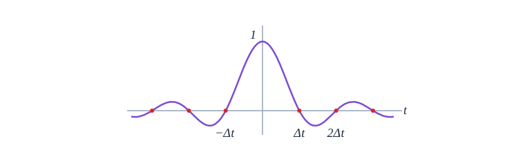
Look closely at $\sin u / u$. It is shifted to the node $k \Delta t$ and stretched so that its zeros land on all the other nodes of the grid: at its own node it equals one, at every other node — zero (fig. 4). This already shows why the series is built the way it is: at any node $t$​${} = m \Delta t$ every term but one vanishes, and the sole survivor — the term with $k$​${} = m$ — yields exactly $y(m \Delta t)$. The series is guaranteed to pass through all the samples.

Here is how it looks on the signal of fig. 3. The slider adds the terms of the series (12) one at a time: every sample brings its own $\sin u / u$ scaled by the sample value, and the sum of these terms assembles step by step into the original signal. We have only seven samples while the series is infinite, so near the ends of the interval the reconstructed curve departs from the original one — the price of truncating the series.