Reduction strategies

The rule that picks the next redex among all the redexes of a term is called a reduction strategy. Let us see where the choice arises. A term has one of three forms:

• a variable $x$ — nothing to reduce;
• an abstraction $\lambda x.M$ — no choice: we reduce the body $M$;
• an application $M\,N$ — redexes may sit both in the left part and in the right one; choosing between them is exactly what a strategy does.

Let us unfold an application: its left part may itself be an application, the left part of that one too, and so on. Descending along the left branches to the first non-application — the head of the term — we get one of two shapes:

In the first shape the head is a variable $x$: there is nothing to contract on the left, redexes can hide only in the arguments $N_i$. In the second the head is an abstraction, and $(\lambda x.M)\,N_1$ is a redex; here is the fork: contract it right away or evaluate the argument first. This choice is what distinguishes the two classic strategies.

The normal strategy contracts the leftmost outermost redex — in our notation $(\lambda x.M)\,N_1$: arguments are substituted into the body unevaluated. The applicative strategy does the opposite: it first brings the argument of the redex to normal form and only then contracts the redex itself.

A term is conveniently drawn as a tree. For example, for $((\lambda x.M)\,N_1)\,N_2$ it looks like this (fig. 1.4): the $@$ nodes are applications, the $\lambda x$ node is an abstraction. The leftmost outermost redex is found on the tree by descending from the root along the left edges: it is the first $@$ whose left child is an abstraction.

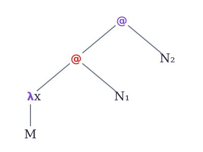
The same descent lets us introduce an important notion — the head normal form. Let us explain it with two examples:

The first term is a head normal form: the descent along the left branches ends at the variable $y$, called the head variable. The head of such a term will never change; redexes can hide only in the arguments $N_i$. The second term is not a head normal form: its head is the redex $(\lambda z.M)\,N_1$, called the head redex.

Let us state both strategies precisely, as rules of an operational semantics. As if we had not enough notions already — we need three more, three syntactic categories. The first is the non-abstraction $\mathit{NA}$:

Here everything seems clear: it is any term except an abstraction. $M$ and $N$ are arbitrary terms, so a non-abstraction may well be a redex — for example $(\lambda y.y)\,z$. The other two categories describe finished results: normal forms $\mathit{NF}$ and their subclass, non-abstraction normal forms $\mathit{NANF}$:

The split is necessary: without it we could form an application with an abstraction on the left — and such a term is not a normal form any more, it is a redex. Examples of $\mathit{NF}$: $\lambda x.\,x$, $\lambda f.\lambda x.\,f\,x$. Examples of $\mathit{NANF}$: $x$, $f\,x$, $x\,(\lambda y.y)\,z$ — and each of them is at the same time an $\mathit{NF}$.

Now, at last, the strategies. At the heart of each lies its own redex-contraction rule. The normal strategy uses ordinary $\beta$-reduction: the redex is contracted right away, the argument $N$ is an arbitrary term and is substituted into the body unevaluated:

The applicative strategy contracts a redex differently — only once the argument has been evaluated, that is, brought to normal form — to the left of the arrow stands an $\mathit{NF}$, and until the argument is one, contraction is forbidden:

Since we cannot contract a redex while the argument is not in normal form, the applicative strategy has a rule for the argument:

The remaining rules are shared by the normal strategy and the applicative one:

The first rule reduces the left part of an application while it remains a non-abstraction; the second moves on to the argument only when the left part is already a $\mathit{NANF}$; the third takes reduction into the body of an abstraction. The categories $\mathit{NA}$ and $\mathit{NANF}$ in the premises are exactly what guarantees the leftmost outermost order: while there is something to contract on the left, we do not look to the right.

The choice of the leftmost outermost redex is no accident: the normalization theorem (Curry) guarantees that if a term has a normal form, then successively contracting exactly such a redex will reach it. For this the normal strategy is called complete.

Completeness is not free: an argument substituted into several places has to be recomputed. For a “big” $N$: $(\lambda x.\,F\,x\,(G\,x)\,x)\,N$ $\to_\beta F\,N\,(G\,N)\,N$ — here $N$ has to be reduced three times — once per copy. The applicative strategy evaluates $N$ exactly once, but pays for this with completeness. Let $\mathrm{K}$ $\equiv \lambda x y.x$, $\mathrm{I}$ $\equiv \lambda x.x$, and let $\Omega$ $\equiv (\lambda x.x\,x)\,(\lambda x.x\,x)$ — a term with no normal form. The normal strategy computes $\mathrm{K}\,\mathrm{I}\,\Omega$ $\twoheadrightarrow_\beta \mathrm{I}$, discarding $\Omega$ without a glance; the applicative one first takes on the argument $\Omega$ — and loops forever.

In programming languages the two strategies live under different names. The applicative one is the call-by-value of strict languages such as C: arguments first, then the application. The normal one underlies lazy languages such as Haskell: call-by-name.