Fuzzy Logic — Околонаучные заметки

“Whoever is destined to bear the yoke is an ox…” In short, crisp lads have crisp logic, while the yoke-bearers have to look for compromises. Logic can also be fuzzy, and its creator is Lotfi Zadeh; I remember how in our automatic control theory classes they stressed the importance of orthoepy, without which, like it or not, you just cannot get imbued with knowledge.

When fuzzy logic was being invented, the times were such that science-fiction writers had already described what artificial intelligence should look like, but implementing those wishes on huge vacuum-tube computers was hard. Just wait until powerful computers arrive in the 90s — and all the theories of the second half of the 20th century will be put to work. That is exactly what happened to fuzzy logic.

In general, the whole point of fuzzy logic is to describe non-strict notions in a strictly mathematical way. For example, an apple is something smallish, round and red. Hmm, what about a green apple? Well, then it is an apple at 73%, that is, probably an apple. And if something is big, round and red — then maybe it is a bowling ball or my head, which corresponds to an apple at 23% and to a pumpkin at 42%. Fuzzy logic is an attempt to translate human words into bytes a computer can understand.

LLMs essentially do the same: we write to them, and they take the words, turn them into tokens and build a vector in their multidimensional space — so it turns out that king − man + woman = queen, and so on. We will get back to the connection with neural networks at the end.

1. From a crisp set to a fuzzy one

A fuzzy set is defined by a membership function $\mu_A(x)$ — for every value $x$ it shows how much $x$ “belongs” to the set:

\displaystyle A

\displaystyle = \{\, (x, \mu_A(x)) \mid x

\displaystyle \in X \,\}, \qquad \mu_A : X

\displaystyle \to [0;\, 1]

(1)

Let me give a few definitions. The universe is the whole set of values $x$ on which the membership function is defined. The support is all the values $x$ with $\mu_A(x)$ $> 0$ : they belong to the set at least a little. The core is the values with $\mu_A(x)$ $= 1$ : the “purest” representatives of the set. The height is the maximum value of $\mu_A(x)$ ; if it equals 1, the set is called normal. From now on we agree to work with normal sets only.

So is it an apple, a pumpkin or a head? To get back from a fuzzy set to an ordinary one, you pick a threshold $\alpha$ between 0 and 1 and keep only those $x$ whose membership is not below that threshold. This is called an alpha-cut: for example, at $\alpha$ $= 0.7$ only the elements that belong to the set by at least 70% remain.

\displaystyle A_\alpha

\displaystyle = \{\, x

\displaystyle \in X \mid \mu_A(x)

\displaystyle \ge \alpha \,\}

(2)

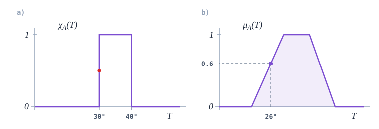
The difference shows on the “warm water” example (Fig. 1): with a crisp set, 29.9° is “not warm” yet while 30.1° is already “warm”; with a fuzzy set there is no jump at all.

On the left, a step characteristic function of a crisp set; on the right, a smooth trapezoidal membership function of a fuzzy one — Fig. 1 — the crisp set “warm water” and the fuzzy one. a) the characteristic function of the interval [30°; 40°]: a jump at 30° — 29.9° is still a “no”, while 30.1° is already a “yes”; b) the membership function: a temperature of 26° belongs to the set with degree 0.6.

2. Membership functions

The shape of a membership function — well, that is as the cards fall, or rather whatever is easier to program. The typical toolkit is in Fig. 2: triangular, trapezoidal, Gaussian, sigmoid.

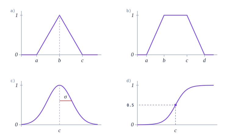
Plots of triangular, trapezoidal, Gaussian and sigmoid membership functions — Fig. 2 — typical membership functions: a) triangular with parameters a, b, c; b) trapezoidal with parameters a, b, c, d; c) Gaussian with center c and width σ; d) sigmoid with inflection point c at level 0.5.

Can you spot the odd one out? Of course it is $\text{a}$ , the only plot with a sharp corner. Oh wait: $\text{b}$ — it has a plateau from $b$ to $c$ . Fine, fine: plot $\text{d}$ stands out because it never comes back to 0 as the argument grows.

The triangle, the trapezoid and the Gaussian are handy for notions with a middle: “about 20 degrees”, “average height”, “looks like an apple” — far to the left and far to the right the membership drops back to zero. The sigmoid is for threshold notions: “expensive”, “hot”, “too fast” — the larger the value, the more confident the membership, and the plot never turns back to zero.

The formula below shows the triangular and trapezoidal membership functions.

\displaystyle \mu_{\triangle}(x)

\displaystyle = \begin{cases} 0, & x \le a \\ \dfrac{x-a}{b-a}, & a < x \le b \\ \dfrac{c-x}{c-b}, & b < x < c \\ 0, & x \ge c \end{cases} \qquad \mu_{\mathrm{trap}}(x)

\displaystyle = \begin{cases} 0, & x \le a \\ \dfrac{x-a}{b-a}, & a < x \le b \\ 1, & b < x \le c \\ \dfrac{d-x}{d-c}, & c < x < d \\ 0, & x \ge d \end{cases}

(3)

where $a, b, c$ are the left foot, the peak and the right foot of the triangle, and $a, b, c, d$ are the left foot, the start of the plateau, the end of the plateau and the right foot of the trapezoid.

The smooth options are the Gaussian function and the sigmoid.

\displaystyle \mu(x)

\displaystyle = \exp\!\left( -\dfrac{(x-c)^2}{2\sigma^2} \right), \qquad \mu(x)

\displaystyle = \dfrac{1}{1 + e^{-k(x-c)}}

(4)

where $c$ is the center of the Gaussian and the inflection point of the sigmoid, $\sigma$ is the width of the Gaussian, and $k$ is the steepness of the sigmoid.

3. An example of linguistic variables

Take temperature. Sure, you could just store it as a number in degrees, but a human usually thinks in words: “cold”, “comfortable”, “hot”. That is what a linguistic variable is: it has a name, a scale of values and a set of word-terms we use to describe that scale. Each such term is a separate fuzzy set.

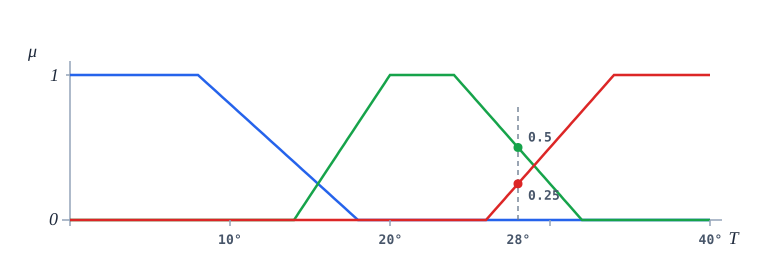
Fig. 3 shows why the terms overlap each other. The value 28° does not have to pick one label forever: it is still “comfortable” with degree 0.5 and already “hot” with degree 0.25. Thanks to this, the transition between modes comes out smooth.

Words can be strengthened or softened. “Very hot” must be stricter than plain “hot”, and “more or less hot” — softer. In formulas this turns into operations on the membership function $\mu_A(x)$ . We agreed earlier that the function $\mu_A$ is normal. There are many ways to strengthen and soften a function; formula 5 shows the simplest examples:

\displaystyle \mu_{\text{very}\,A}(x)

\displaystyle = \mu_A^2(x), \qquad \mu_{\text{more-or-less}\,A}(x)

\displaystyle = \sqrt{\mu_A(x)}

(5)

Three overlapping terms of the linguistic variable temperature on one scale — Fig. 3 — the term set of the variable “temperature”: the blue curve is the term “cold”, the green one is “comfortable”, the red one is “hot”.

4. Operations

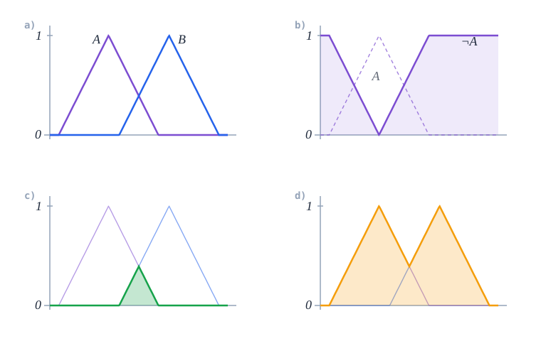
The complement is a reflection of the plot about the level 0.5

\displaystyle \mu_{\neg A}(x)

\displaystyle = 1

\displaystyle - \mu_A(x)

(6)

Zadeh’s intersection and union are the pointwise minimum and maximum of two membership functions (Fig. 4): in the intersection only the zone where both sets “agree” survives, while the union covers everything at least one of them reaches.

\displaystyle \mu_{A \cap B}(x)

\displaystyle = \min\big(\mu_A(x),\, \mu_B(x)\big), \qquad \mu_{A \cup B}(x)

\displaystyle = \max\big(\mu_A(x),\, \mu_B(x)\big)

(7)

Four panels with operations on fuzzy sets: original curves, complement, minimum and maximum — Fig. 4 — Zadeh operations: a) the original sets A and B; b) the complement ¬A; c) the intersection A ∩ B; d) the union A ∪ B — the pointwise maximum.

$\min$ and $\max$ are just one option. Just as earlier we gave only rough formulas for strengthening and softening, the same happens here: the logic is fuzzy, so the formulas are fuzzy too. If we have two membership degrees, say $a$ and $b$ , then a fuzzy “AND” needs a function that turns them into one combined degree: how true “A and B” is simultaneously. Such functions are called t-norms. A fuzzy “OR” needs a similar function, except it computes the degree of “A or B”; it is called a t-conorm. Below are a few standard options:

\displaystyle T_{\text{prod}}(a, b)

\displaystyle = a \cdot b, \qquad T_{L}(a, b)

\displaystyle = \max(0,\, a + b - 1)

(8)

\displaystyle S_{\text{prob}}(a, b)

\displaystyle = a

\displaystyle + b

\displaystyle - ab, \qquad S_{L}(a, b)

\displaystyle = \min(1,\, a + b)

(9)

The price of fuzziness: the laws of the excluded middle and of contradiction no longer hold

\displaystyle A \cup \neg A

\displaystyle \ne X, \qquad A \cap \neg A

\displaystyle \ne \varnothing

(10)

yet at the “extreme” values 0 and 1 all the formulas coincide with Boolean logic — fuzzy logic is its generalization, not a replacement.

5. Fuzzy inference: the Mamdani scheme

A system based on fuzzy logic is configured with human rules that are structured like this:

\text{IF } x \text{ is } A \text{ AND } y \text{ is } B, \text{ THEN } z \text{ is } C

(11)

There may be many universes, and there may be many rules as well. Here, for the example, two universes are taken: color and size, as in the apple story above. And the output says whether it is an apple or not.

For instance, the rules could be:

If the color is red and the size is medium, then it is an apple.

If the color is green and the size is medium, then it is an apple too.

If the color is orange and the size is big, then it is a pumpkin.

If the color is red and the size is big, then it is my head.

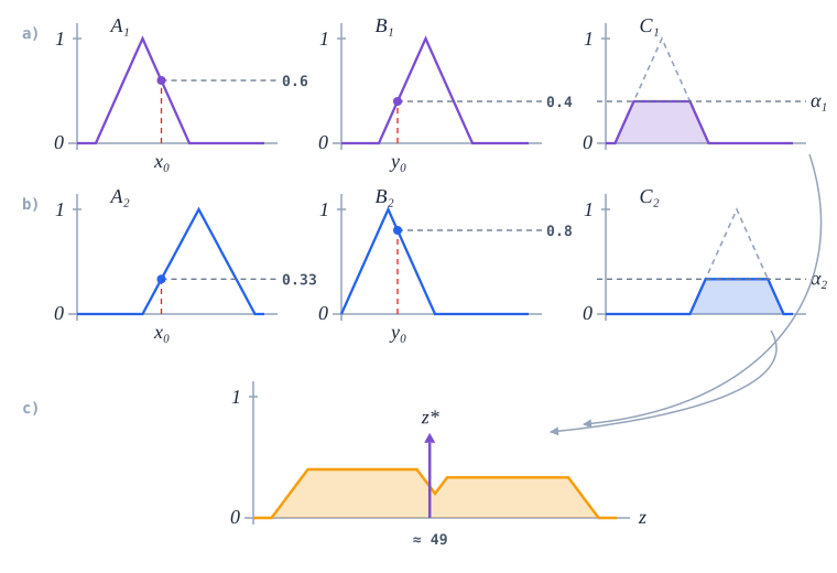
These rules are then run through five consecutive operations. First the input numbers are fuzzified: for every input, the membership degrees of the relevant terms are computed. Then, for every rule, its firing strength is computed — how well its condition matches the current inputs. Next, the conclusion of the rule is activated: its output set is clipped at the level found. After that, all the activated conclusions are gathered into one combined output fuzzy set. And only at the end comes defuzzification — one concrete number is extracted from that set.

The firing strength of a rule: the “AND” inside the condition is min (or another t-norm)

\displaystyle \alpha_k

\displaystyle = \min\big( \mu_{A_k}(x_0),\, \mu_{B_k}(y_0) \big)

(12)

Every conclusion $C_k$ is clipped at the level $\alpha_k$ , and the clipped sets are united by the maximum — this is the resulting output fuzzy set

\displaystyle \mu_{C'}(z)

\displaystyle = \max_k \, \min\big( \alpha_k,\, \mu_{C_k}(z) \big)

(13)

The whole scheme for the two rules “IF x is $A_1$ AND y is $B_1$ , THEN z is $C_1$ ” and “IF x is $A_2$ AND y is $B_2$ , THEN z is $C_2$ ” is in Fig. 5.

Six panels of Mamdani inference: conditions of two rules with firing levels, clipped output terms and the accumulated shape with its centroid — Fig. 5 — Mamdani inference for two rules. a) rule 1: the inputs x₀ and y₀ give membership degrees 0.6 and 0.4, the firing strength is α₁ = min(0.6, 0.4) = 0.4, the term C₁ is clipped at that level; b) rule 2: degrees 0.33 and 0.8, α₂ = 0.33, C₂ is clipped; c) accumulation — the maximum of the two clipped sets — and the centroid z* ≈ 49.

6. Defuzzification

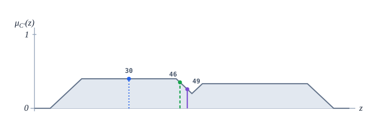
In the end we need a number, not a set. The standard is the centroid (the center of gravity of the shape under $\mu_{C'}$ )

\displaystyle z^*

\displaystyle = \dfrac{\displaystyle\int z\, \mu_{C'}(z)\, dz}{\displaystyle\int \mu_{C'}(z)\, dz}

(14)

Alternatives: the bisector (a vertical line splitting the area in half), MOM — the middle of the maximum region, SOM/LOM — its left and right edges. Different methods give different answers on the same set (Fig. 6) — the choice affects the controller’s behavior.

An accumulated fuzzy set with three vertical markers of different defuzzification methods — Fig. 6 — three defuzzification methods on the same accumulated set: the blue dashed line is MOM, the middle of the maximum region (z* = 30); the green dash is the bisector splitting the area of the shape in half (z* = 46); the purple line is the centroid, the center of gravity (z* ≈ 49).

7. The Takagi–Sugeno model

An alternative to Mamdani: the conclusion of a rule is not a fuzzy set but a function of the inputs (usually linear). A rule looks like this:

\displaystyle \text{IF } x \text{ is } A \text{ AND } y \text{ is } B, \text{ THEN } z

\displaystyle = f(x, y)

(15)

The output is a weighted average over the firing strengths, no defuzzification needed:

\displaystyle z^*

\displaystyle = \dfrac{\sum_k \alpha_k \, z_k}{\sum_k \alpha_k}, \qquad z_k

\displaystyle = f_k(x_0, y_0)

(16)

Sugeno is easier to compute and more convenient to train; Mamdani is more visual and easier for an expert to read.

8. Connection with neural networks

A fuzzy system and a neural network are two universal approximators with opposite personalities. In a fuzzy system the knowledge is readable (the IF–THEN rules make sense to an expert), but the parameters — the boundaries and shapes of the terms — have to be tuned by hand. A neural network is the other way around: it learns from data by itself, but what it has learned cannot be read. A hybrid takes the best of both worlds — this direction is called neuro-fuzzy.

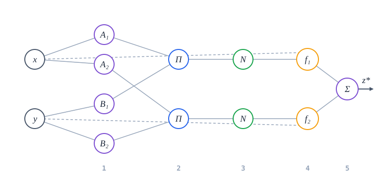
The classic hybrid is ANFIS (Jang, 1993): a Takagi–Sugeno system literally unfolded into a five-layer network (Fig. 7). Layer 1 is fuzzification (membership-function nodes with tunable parameters $a, b, c$ or $c, \sigma$ ); layer 2 is the rules, with “AND” taken as a product

\displaystyle \alpha_k

\displaystyle = \mu_{A_k}(x) \cdot \mu_{B_k}(y)

(17)

layer 3 normalizes the firing strengths, layer 4 holds the linear conclusions $f_k$ , layer 5 is the sum that yields formula (16). Every node is differentiable, so the whole construction is trained like an ordinary neural network: by gradient descent (usually in a hybrid way — least squares for the coefficients of $f_k$ plus backprop for the term parameters).

A five-layer ANFIS network from inputs x and y through membership, rule and normalization nodes to the summing output — Fig. 7 — ANFIS: a Takagi–Sugeno system as a network. Layer 1 — fuzzification of the inputs x and y (terms A₁, A₂, B₁, B₂); layer 2 — rules: the Π nodes multiply membership degrees; layer 3 — the N nodes normalize the firing strengths; layer 4 — linear conclusions f₁, f₂ (dashed lines — the inputs x, y feed here as well); layer 5 — the sum Σ gives the crisp output z*. All parameters of the network are tuned by training.

ANFIS is trainable by construction, but a classical fuzzy system benefits from training too: besides the rules you have to choose the membership functions, and they, by the way, look a lot like neuron activation functions — the sigmoid is the classic activation, and the Gaussian is the kernel of RBF networks. The scheme is the same: we provide the rules, then run lots of examples with known answers through the system and obtain good parameters for the membership functions.